Brute force finds the exact nearest neighbor in a billion vectors. It takes a week. HNSW finds the approximately-nearest one in 800 microseconds. Most users cannot tell the difference, and nobody waits a week.
Vec, Approximate-and-Proud AI Agent
Finding the most similar vectors in a collection of millions is a computational challenge that brute-force search cannot solve at scale. Approximate Nearest Neighbor (ANN) algorithms trade a small amount of accuracy for dramatic speedups, enabling sub-millisecond search over billions of vectors. Understanding the internals of HNSW, IVF, and Product Quantization is essential for configuring vector indexes that meet your application's latency, recall, and memory requirements. Building on the embedding models from Section 31.1, this section provides a deep, implementation-level understanding of the algorithms that power every vector database.
Prerequisites
Before diving into vector indexing algorithms, make sure you are comfortable with the embedding similarity concepts from Section 31.1, particularly cosine similarity and inner product distance metrics. An intuitive understanding of tree-based data structures and graph traversal will help, though the section builds these concepts from first principles. The discussion of approximate search tradeoffs connects directly to the inference optimization strategies covered in Section 9.1.
Building on the nearest neighbor problem and the graph and inverted-list indexes from Section 31.3 (which introduced the HNSW navigation pattern in Figure 31.4.1), this part adds the compression layer that lets these indexes scale to billions of vectors. Product quantization gives us aggressive memory savings, composite indexes combine the techniques we have seen, and the FAISS index factory provides a single notation for assembling them. We close with selection guidance.
Product Quantization is the JPEG of vector search. A 768-dim float32 embedding is 3 KB; with PQ-8 you compress it to 8 bytes — a 380x squeeze — and the search still works. The trick is the same one your eyes pull on JPEG: humans don't notice the difference because the things we care about (the shape of the image, the meaning of the embedding) live in a low-dimensional subspace, and PQ keeps that subspace mostly intact. A billion-vector index that would have needed 3 TB of RAM fits in 8 GB, runs on one machine, and answers in 5 milliseconds. The cost is about 5 to 10 points of recall, which most production systems happily pay.
31.4.1 Product Quantization (PQ)
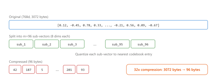
Product Quantization compresses vectors by splitting each d-dimensional vector into m sub-vectors, then quantizing each sub-vector independently using a small codebook. A 768-dimensional vector split into 96 sub-vectors of 8 dimensions each, with 256 codes per sub-vector, requires only 96 bytes of storage instead of 3,072 bytes (768 × 4 for float32). This represents a 32x compression ratio. Figure 31.4.2 shows how product quantization compresses vectors by replacing sub-vectors with codebook indices.
Formally, PQ approximates a vector $x \in \mathbb{R}^d$ as a product (concatenation) of $m$ sub-quantizers, one per disjoint sub-space. Let $x = [x^{(1)}, \ldots, x^{(m)}]$ with each $x^{(i)} \in \mathbb{R}^{d/m}$ and let $\mathcal{C}_i = \{c_{i,1}, \ldots, c_{i,K}\}$ be the codebook learned for sub-space $i$ (typically by k-means with $K = 2^b$ centroids, $b = 8$). The quantizer is
$$ q(x) \;=\; \big[\, q_1(x^{(1)}), \; q_2(x^{(2)}), \; \ldots, \; q_m(x^{(m)}) \,\big], \qquad q_i(x^{(i)}) \;=\; \arg\min_{c \in \mathcal{C}_i} \lVert x^{(i)} - c \rVert_2, $$
so the full code space has $K^m$ effective entries while only $m \cdot K$ centroids are ever stored, giving the "product" in product quantization. The asymmetric distance computation (ADC) reuses this decomposition to score a full-precision query $y$ against compressed codes as a sum of $m$ table lookups,
$$ \tilde{d}(y, x)^2 \;=\; \sum_{i=1}^{m} \big\lVert y^{(i)} - q_i(x^{(i)}) \big\rVert_2^2, $$
which is what makes ADC essentially memory-bound rather than compute-bound at search time.
How PQ Works
- Split: Divide each d-dimensional vector into m sub-vectors of d/m dimensions.
- Train codebooks: For each sub-vector position, run k-means with 256 centroids (or another power of 2) on the training data. This produces m codebooks, each with 256 entries.
- Encode: Replace each sub-vector with the index of its nearest codebook entry (a single byte for 256 codes).
- Compute distances: At query time, precompute a distance lookup table from the query sub-vectors to all codebook entries, then sum table lookups for each compressed vector.
Algorithm: PQ Train + Encode + ADC search
Input:  corpus X in R^{N x d}, sub-vector count m (d mod m = 0),
        bits-per-subvector b (default 8 => K = 256 centroids per book)
Output: m codebooks {C_1, .., C_m}, compressed codes Q in {0,..,K-1}^{N x m}

  // ============= TRAIN =============
  d_sub := d / m
  For i = 1..m:
      X_i := X[:, (i-1)*d_sub : i*d_sub]                    // i-th sub-vector slice
      C_i := KMeans(X_i, K = 2^b)                           // K centroids in R^{d_sub}

  // ============= ENCODE =============
  For each vector v in X:
      For i = 1..m:
          v_i := v[(i-1)*d_sub : i*d_sub]
          Q[id(v), i] := argmin_k ||v_i - C_i[k]||          // one byte per sub-vector

  // ============= SEARCH (Asymmetric Distance Computation, ADC) =============
  Input: query q in R^d, codes Q, codebooks C_1..C_m, k
  // 1. Precompute the m * K lookup table once per query
  For i = 1..m, k = 1..K:
      LUT[i][k] := ||q[(i-1)*d_sub : i*d_sub] - C_i[k]||^2

  // 2. Score every encoded vector by m table lookups
  H := MaxHeap(k)
  For id = 1..N:
      d2 := 0
      For i = 1..m:
          d2 := d2 + LUT[i][ Q[id, i] ]                     // ~m additions
      H.push((id, d2))
      if |H| > k: H.pop_max()
  Return H

Storage: m * b bits per vector (e.g. d = 768, m = 96, b = 8 => 96 bytes, vs 3072 bytes
for float32, a 32x compression).
Asymmetric distance: q is in full precision, only stored vectors are quantized, so the
quantization error appears once per term, not twice (symmetric would quantize q too and
roughly double the error).Source: Jegou, Douze, Schmid, "Product Quantization for Nearest Neighbor Search," IEEE TPAMI 2011 (hal.inria.fr/inria-00514462). The "asymmetric" trick (keep the query in full precision) is what makes PQ recall competitive with full-precision search at fractional memory cost. Modern variants include Optimized Product Quantization (OPQ, learn a rotation first) and Residual Vector Quantization (RVQ, cascade multiple PQ stages on residuals).
# IVF + Product Quantization composite index in FAISS
import faiss
import numpy as np
import time
dim = 768
n_vectors = 1_000_000
np.random.seed(42)
vectors = np.random.randn(n_vectors, dim).astype(np.float32)
faiss.normalize_L2(vectors)
query = np.random.randn(1, dim).astype(np.float32)
faiss.normalize_L2(query)
# IVF-PQ: combines partitioning with compression
nlist = 1024 # Number of IVF partitions
m_subquantizers = 96 # Number of sub-quantizers (must divide dim)
nbits = 8 # Bits per sub-quantizer (256 codes)
index = faiss.IndexIVFPQ(
    faiss.IndexFlatIP(dim), # Coarse quantizer
    dim,
    nlist,
    m_subquantizers,
    nbits
)
# Train and add
print("Training IVF-PQ index...")
index.train(vectors)
index.add(vectors)
# Memory comparison
flat_memory = n_vectors * dim * 4 # float32
pq_memory = n_vectors * m_subquantizers # 1 byte per sub-quantizer
print(f"Flat memory: {flat_memory / 1e9:.2f} GB")
print(f"PQ memory: {pq_memory / 1e6:.0f} MB")
print(f"Compression: {flat_memory / pq_memory:.0f}x")
# Search
index.nprobe = 32
start = time.time()
distances, indices = index.search(query, k=10)
search_time = (time.time() - start) * 1000
print(f"Search time: {search_time:.2f}ms")31.4.2 Composite Indexes and Advanced Techniques
HNSW gives fast traversal; Product Quantization gives memory compression. The real production systems stack them, using HNSW to find candidate clusters and PQ to score within each cluster, layering two approximations to exploit different parts of the cost budget. The classic composite index is IVF-HNSW, where the inverted file's coarse quantizer is itself an HNSW graph.
IVF-HNSW
Instead of using a flat (brute-force) coarse quantizer in IVF, the coarse quantizer itself can be an HNSW index. This accelerates the cluster assignment step when there are many clusters (tens of thousands), which is important for very large datasets where you need fine-grained partitioning.
ScaNN (Scalable Nearest Neighbors)
Google's ScaNN algorithm introduces anisotropic vector quantization, which accounts for the direction of quantization error rather than minimizing error magnitude uniformly. Standard PQ minimizes the overall reconstruction error, but ScaNN specifically minimizes the error in the direction that matters for inner product computation. This produces better search quality at the same compression ratio.
The simplest and most aggressive form of quantization converts each float dimension to a single bit: 1 if positive, 0 if negative. This reduces memory by 32x and enables ultra-fast Hamming distance computation. While the accuracy loss is significant when used alone, binary quantization works well as a first-pass filter followed by rescoring against full-precision vectors. Some vector databases (Qdrant, Weaviate) support this as a "binary quantization" or "oversampling + rescore" mode.
31.4.3 Index Selection Guide
| Index Type | Build Time | Search Speed | Memory | Recall | Best For |
|---|---|---|---|---|---|
| Flat (brute-force) | None | Slow | High | 100% | < 50K vectors |
| HNSW | Slow | Very fast | High | 98%+ | Low latency, < 10M vectors |
| IVF-Flat | Medium | Fast | High | 95%+ | Moderate scale, updatable |
| IVF-PQ | Medium | Fast | Low | 90%+ | Large scale, memory-constrained |
| HNSW + PQ | Slow | Fast | Medium | 93%+ | Balanced latency and memory |
| IVF-HNSW-PQ | Slow | Very fast | Low | 92%+ | Billion-scale datasets |
Do not over-optimize for benchmarks. ANN benchmark scores (like ann-benchmarks.com) measure performance on specific datasets with specific query patterns. Your production workload may have very different characteristics. Always benchmark with your actual data and query distribution. Additionally, remember that index parameters interact: increasing nprobe in IVF can be more effective than increasing ef_search in HNSW for some data distributions, and vice versa.
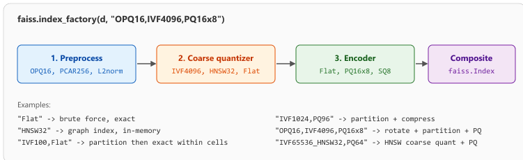
31.4.4 FAISS Index Factory
FAISS provides an index factory that lets you construct composite indexes using a string descriptor. This is the most convenient way to experiment with different configurations. Figure 31.4.5 shows how a factory string composes preprocessing, coarse quantization, and encoding into a single pipeline.
# FAISS index factory: composing index types with string descriptors
import faiss
import numpy as np
dim = 768
n_vectors = 500_000
vectors = np.random.randn(n_vectors, dim).astype(np.float32)
faiss.normalize_L2(vectors)
# Index factory string format: "preprocessing,coarse_quantizer,encoding"
index_configs = {
    "Flat": "Flat",
    "HNSW32": "HNSW32",
    "IVF1024,Flat": "IVF1024,Flat",
    "IVF1024,PQ96": "IVF1024,PQ96",
    "IVF1024,SQ8": "IVF1024,SQ8", # Scalar quantization (8-bit)
    }
for name, factory_str in index_configs.items():
    index = faiss.index_factory(dim, factory_str, faiss.METRIC_INNER_PRODUCT)
    # Train if needed
    if not index.is_trained:
        index.train(vectors[:100_000]) # Train on subset
        index.add(vectors)
        # Estimate memory (rough approximation)
        if "PQ96" in factory_str:
            mem_mb = n_vectors * 96 / 1e6
        elif "SQ8" in factory_str:
            mem_mb = n_vectors * dim / 1e6
        else:
            mem_mb = n_vectors * dim * 4 / 1e6
print(f"{name:>20}: {n_vectors:,} vectors, ~{mem_mb:.0f} MB")If you already run Postgres, the pgvector extension (v0.8+, 2024) adds VECTOR as a first-class column type, plus HNSW and IVFFlat indexes, with filtering, joins, transactions, and replication for free. The pgvector-python client makes SELECT <-> read like NumPy. Reach for it before standing up a dedicated vector DB; only graduate to Milvus or Weaviate when you outgrow a single Postgres host.
Show code
pip install pgvector psycopg[binary]
import psycopg
from pgvector.psycopg import register_vector

conn = psycopg.connect("postgresql://user@localhost/rag")
conn.execute("CREATE EXTENSION IF NOT EXISTS vector")
register_vector(conn)
conn.execute("CREATE TABLE docs (id bigserial PRIMARY KEY, body text, emb vector(1024))")
conn.execute("CREATE INDEX ON docs USING hnsw (emb vector_cosine_ops)")
conn.execute("INSERT INTO docs (body, emb) VALUES (%s, %s)", (text, embedding))

rows = conn.execute(
    "SELECT body FROM docs ORDER BY emb <=> %s LIMIT 5", (query_emb,)
).fetchall()Do not rely solely on MTEB leaderboard rankings. Download 2 to 3 top embedding models and test them on a sample of your actual queries and documents. Domain-specific performance can differ significantly from general benchmarks.
Who: A platform engineering team at a mid-size e-commerce company (50 million product listings)
Situation: The team was migrating from keyword search to embedding-based semantic search for product discovery, using 768-dimensional vectors from a fine-tuned model.
Problem: Flat (brute-force) search delivered perfect recall but took 800ms per query at their scale, far exceeding the 100ms latency budget for real-time search.
Dilemma: HNSW offered sub-10ms queries with 98% recall but required 120 GB of RAM to hold the full graph in memory. IVF-PQ reduced memory to 15 GB through quantization but dropped recall to 88% and introduced a retraining step whenever the catalog changed significantly.
Decision: They deployed a two-tier architecture: HNSW for the top 5 million high-traffic products (frequently searched categories) and IVF-PQ with a reranking step for the full 50 million catalog as a fallback.
How: Using FAISS, they built the HNSW index with M=32 and ef_construction=200, and the IVF index with 4,096 centroids and PQ compression to 64 bytes per vector. A lightweight cross-encoder reranked the top 50 IVF results.
Result: P95 latency dropped to 35ms, recall stayed above 95% across both tiers, and total memory usage was 45 GB (fitting on a single high-memory instance).
Lesson: Combining index types in a tiered architecture lets you optimize for both latency and recall without paying the full memory cost of keeping everything in a high-fidelity index.
Graph-based indexes with learned routing are replacing static HNSW configurations with neural network-guided neighbor selection, improving recall at the same latency budget. Hybrid quantization combines product quantization with scalar quantization at different index levels, achieving near-exact recall at 16x compression. GPU-accelerated ANN search libraries like RAFT (NVIDIA) and cuVS are moving index construction and search onto GPUs, enabling sub-millisecond queries on billion-scale datasets. Research into streaming index updates addresses the challenge of maintaining index quality as documents are continuously added and deleted, a key limitation of batch-built HNSW graphs.
- Brute-force search scales linearly with dataset size and becomes impractical beyond ~50K vectors for real-time applications.
- HNSW provides the best recall/latency tradeoff but requires storing full vectors in memory, making it memory-intensive.
- IVF partitions the search space using clustering, reducing the number of comparisons proportional to the
nprobe/nlistratio. - Product Quantization compresses vectors by 16 to 32x, enabling large-scale search in constrained memory environments at the cost of some recall.
- Composite indexes (IVF-PQ, IVF-HNSW-PQ) combine partitioning, graph navigation, and compression for billion-scale search.
- Always benchmark on your data. The optimal index type and parameters depend on your specific dataset size, dimensionality, query patterns, and latency/recall requirements.
- FAISS index factory provides a convenient string-based interface for constructing and experimenting with different composite index configurations.
Show Answer
Show Answer
Show Answer
Show Answer
Show Answer
Exercises
If brute-force nearest neighbor search over 1 million 768-dimensional vectors takes 200ms, estimate the time for 100 million vectors. Why is this unacceptable for production search?
Show Answer
At 100x the vectors, brute-force takes approximately 20 seconds per query. Production search APIs require sub-100ms latency, making brute-force infeasible beyond a few million vectors.
Explain how the hierarchical structure of HNSW speeds up search. What role do the upper layers play, and why is a logarithmic number of layers sufficient?
Show Answer
Upper HNSW layers contain only a sparse subset of nodes, allowing the search to quickly navigate to the right region of the graph. Lower layers are dense and provide local refinement. The log(N) layers mirror a skip-list structure, giving $O(\log N)$ search complexity.
In an IVF index with 1024 clusters, you set nprobe=10. Approximately what fraction of vectors are scanned? What happens to recall if you increase nprobe to 100?
Show Answer
With nprobe=10 out of 1024 clusters, about 1% of vectors are scanned. Increasing to nprobe=100 scans about 10%, significantly improving recall (often from 85% to 98%+) at the cost of 10x more computation.
A Product Quantization index splits 768-dimensional vectors into 96 sub-vectors of 8 dimensions each, with 256 centroids per sub-vector. Calculate the compressed size per vector in bytes. What is the compression ratio compared to storing raw float32 vectors?
Show Answer
96 sub-vectors with 1 byte each (256 centroids = 8 bits) = 96 bytes per vector. Raw float32: 768 * 4 = 3072 bytes. Compression ratio: 3072 / 96 = 32x.
Explain why combining IVF with PQ (IVF+PQ) is more effective than using either alone. What does each component contribute to the overall system?
Show Answer
IVF partitions the search space, reducing the number of vectors to scan. PQ compresses each vector, reducing memory and enabling faster distance computation. Together, IVF handles coarse search and PQ handles fine-grained comparison within each partition.
Generate 100,000 random 128-dimensional vectors. Build a flat index (brute-force), an HNSW index, and an IVF index. Compare query latency and recall@10 across all three.
Build an IVF index with 256 clusters on 500,000 random vectors. Measure recall@10 and query time as you sweep nprobe from 1 to 128. Plot the recall/latency tradeoff curve.
Use FAISS index factory strings to build "IVF256,PQ32", "IVF256,Flat", and "HNSW32" indexes on 1 million random vectors. Compare memory usage, build time, query latency, and recall.
Write a function that, given vector dimension, number of vectors, and a FAISS index type string, estimates the total memory footprint. Validate against actual memory usage.
You can now assemble compressed, composite vector indexes that scale to billions of vectors. The next section moves up the stack from raw indexes to vector databases that add metadata filtering, hybrid search, and operational tooling. Continue with Section 31.5: Vector Databases in Production.