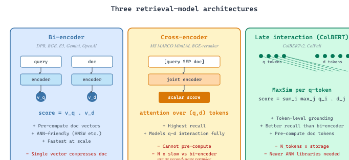
This section catalogs the embedding and reranking models that power retrieval-augmented generation in 2026. An embedding model maps a query or document into a fixed-length vector so that semantically similar items end up close to each other; a reranker then re-scores the top-k candidates returned by the embedding-based search with a heavier cross-encoder pass to maximize relevance. The section compares three architectural families: bi-encoders (separate query and document towers, ANN-friendly), cross-encoders (joint encoding, slower but more accurate), and ColBERT-style late-interaction models (per-token vectors plus MaxSim). For each, we name the dominant closed-API and open-weight choices, their multilingual and multimodal coverage, and the licensing constraints that matter when shipping to production. For the underlying contrastive training, see Section 31.1.
"Change the embedder, re-encode the corpus. Pick the model after the eval set, never before; the leaderboards shortlist three, and your data picks one."
Vec, Dimensionally-Particular AI Agent
The 2026 embedding-model landscape sorts into four camps. Closed-API embedders (OpenAI text-embedding-3, Cohere Embed v3 / Embed-4, Voyage AI voyage-3) are the easiest path with strong multilingual support and per-call pricing. Open-weight embedders (BGE-M3, NV-Embed, GTE-Qwen2, Stella, Snowflake Arctic Embed, mxbai-embed, Linq-Embed-Mistral, Jina Embeddings v3) are the self-host path with similar quality and full control of the model. Late-interaction embedders (ColBERTv2, ColPali, JinaColBERT) emit per-token vectors for higher recall on hard queries. And multimodal embedders (ColPali for documents, Cohere Embed v3 multimodal, JinaCLIP, Voyage multimodal) handle images and document layouts directly. The choice axes are dimension count (affects vector-store cost), license (closed APIs vs Apache 2.0 vs research-only), context length (512 vs 8K vs 32K), language coverage, and whether you need the matryoshka property that lets you truncate the vector at query time.
Prerequisites
This section assumes the embedding-model architectures from Section 3.1, the open-versus-closed licensing landscape from Section 10.6, and the multilingual considerations from Section 32.4.
Pick the model after you have an in-domain eval set; pick it before you ingest a corpus, because the embedder defines the vectors and changing the embedder forces a full re-encode. The leaderboards (Section 36.3) shortlist the candidates; your eval set decides between the top three. The dimension count, license, and context length below are 2026-accurate but change quarterly; always check the model card for the current state.
36.4.1 Closed-API embedders
Closed APIs are the fastest path to retrieval that works. You pay per token (or per call), the model is opaque, and you cannot self-host. The 2026 standouts:
- OpenAI text-embedding-3-large and text-embedding-3-small (OpenAI, 2024): the OpenAI third-generation embedders. text-embedding-3-large emits 3072-dimensional vectors at $0.13 per 1M tokens; text-embedding-3-small emits 1536-dimensional vectors at $0.02 per 1M tokens. Both support the
dimensionsparameter for Matryoshka-style truncation down to 256 dimensions with minimal quality loss. Training data is undisclosed; context length is 8191 tokens; license is API-only. Pick text-embedding-3-large when budget allows and you want the highest closed-API score; pick text-embedding-3-small when cost-per-vector matters and the quality gap (3-5 points on MTEB) is acceptable. The dimensions parameter is the most underused feature: settingdimensions=512on text-embedding-3-large saves 6x storage with a 1-2 point quality drop, often a net win. - Cohere Embed v3 and Embed-4 (Cohere, 2023; v4 in late 2024-25): Cohere's hosted embedders, distinguished by per-call
input_typehints (search_query, search_document, classification, clustering) that route the input through type-specific transformations. Embed v3 emits 1024-dimensional vectors at $0.10 per 1M tokens; Embed-4 emits 1024-dimensional matryoshka-trainable vectors with stronger multilingual scores on MIRACL. Both support 100+ languages with closer-to-equal quality across them than OpenAI's. Context length is 512 tokens (a real limitation on long documents; chunk first). License is API-only with on-prem options for enterprise tier. Pick Cohere Embed when multilingual breadth matters or when the input_type hints make a measurable difference (they do for query-document asymmetry); the 512-token context is the main thing to plan around. - Voyage AI voyage-3-large and voyage-3 (Voyage AI, 2024-25): Voyage's flagship general-purpose embedders, distinguished by domain-tuned variants (voyage-code-3, voyage-finance-2, voyage-law-2, voyage-multimodal-3) that score 5-15 points higher than the general model on in-domain benchmarks. voyage-3-large emits 1024-dimensional vectors with a 32K context (the longest in the closed-API space) at $0.18 per 1M tokens. License is API-only. Pick Voyage when your corpus is in one of the supported verticals or when the 32K context is required (e.g., long-form contracts, scientific papers); for general corpora at lower cost, OpenAI or Cohere are alternatives. The matryoshka-trained dimensions parameter and the 32K context together cover 90% of long-document RAG without re-chunking.
- Mistral-Embed (Mistral AI, 2024): Mistral's hosted embedder, 1024-dimensional, 8K context, competitive multilingual quality, $0.10 per 1M tokens. License is API-only; the underlying model is not open-weights (unlike most Mistral generative models). Pick Mistral-Embed when you are already on Mistral La Plateforme and want a coherent stack; the differentiation against Cohere and Voyage is small.
- Google Gemini Embedding (text-embedding-004 / gemini-embedding-001) (Google, 2024-25): Google's hosted embedder, 768-dimensional default with matryoshka support down to 256, multilingual, 2048-token context. License is API-only. Pick Gemini Embedding when you are already on Google Cloud and want first-party integration with Vertex AI and BigQuery vector search.
36.4.2 Open-weight embedders
Open-weight embedders are the right pick when self-hosting is required, when per-call API cost would dominate at scale, or when the model card needs to be inspectable. The 2026 leaders, mostly Apache 2.0 or MIT, runnable on a single 24GB GPU at production batch sizes:
- BGE-M3 (BAAI, 2024) is the BAAI multifunctional embedder, distinguished by emitting dense, sparse (BM25-replacing), and ColBERT-style multi-vector outputs in a single forward pass. Dense vectors are 1024-dimensional; sparse vectors are vocab-sized; multi-vector is 8 token vectors. Context length is 8192 tokens; trained on 100+ languages; license is MIT. The 2024 hybrid-retrieval consensus is built largely on BGE-M3's three-output design. Pick BGE-M3 as the open-weight default in 2026 for any team that wants hybrid retrieval without integrating multiple models; the model is large (570M parameters) but the inference cost is paid once per document.
- NV-Embed-v2 (NVIDIA, 2024) is NVIDIA's open embedder built on Mistral-7B as the encoder backbone, distinguished by frequently topping the MTEB English leaderboard in 2024-25. Emits 4096-dimensional vectors (cuttable via matryoshka to 1024 or 512); context length 32K tokens; license is CC-BY-NC-4.0 (non-commercial only). Pick NV-Embed-v2 for research or for licensed commercial use through NVIDIA AI Enterprise; for permissive-license production, BGE-M3 or GTE-Qwen2 are alternatives. The 4096-dimension default is large enough that storage cost is a real factor; matryoshka truncation to 1024 dimensions costs only 1-2 MTEB points.
- GTE-Qwen2-7B-instruct (Alibaba, 2024): Alibaba's General Text Embeddings family built on Qwen2-7B with instruction tuning, distinguished by 32K-context support and strong multilingual numbers. Vectors are 3584-dimensional; license is Apache 2.0. Pick GTE-Qwen2-7B when you want a 7B-parameter open embedder with long context under a permissive license; the inference cost is meaningfully higher than BGE-M3 because of the parameter count.
- Stella en 1.5B v5 and Stella_en_400M_v5 (Dun Zhang, 2024): open embedders distinguished by very strong MTEB scores per parameter (Stella 1.5B is competitive with NV-Embed-7B on English MTEB at 1/5 the size). Vectors are 1024-dimensional matryoshka-trained; license is MIT. Pick Stella when you want top-tier MTEB at lower inference cost than NV-Embed; the multilingual story is weaker than BGE-M3.
- Snowflake Arctic Embed L 2.0 and M 2.0 (Snowflake, 2024): Snowflake's open embedders, distinguished by very strong recall-per-dimension (the 2.0 line was the first open embedder competitive with closed APIs on Snowflake's own enterprise retrieval benchmarks). Vectors are 1024-dimensional matryoshka-trained; license is Apache 2.0; context length 8K. Pick Arctic Embed when Snowflake-ecosystem integration matters or when you want a top-3 open MTEB scorer; for the same architecture without Snowflake's vertical tuning, Stella is the lighter alternative.
- mxbai-embed-large-v1 (Mixedbread, 2024): Mixedbread's open embedder, distinguished by very strong English-only MTEB scores at a small (335M parameter) size. Vectors are 1024-dimensional matryoshka-trained; license is Apache 2.0; context length 512. Pick mxbai-embed when you want a small, fast, English-only open embedder; the 512-context limit and the English focus are the two things to plan around.
- Linq-Embed-Mistral (Linq AI Research, 2024): open embedder built on Mistral-7B-Instruct backbone, distinguished by topping the MTEB English leaderboard at release. Vectors are 4096-dimensional; license is Apache 2.0; context length 32K. Pick Linq-Embed-Mistral when you want a Mistral-lineage open embedder with permissive license and the storage cost of 4096 dimensions is acceptable.
- Jina Embeddings v3 (Jina AI, 2024): Jina's open embedder, distinguished by task-specific LoRA adapters (retrieval.query, retrieval.passage, separation, classification, text-matching) that route the input through different LoRA paths inside a 570M backbone. Vectors are 1024-dimensional matryoshka-trained down to 32; license is CC-BY-NC-4.0 (commercial requires API or license); context length 8K. Pick Jina Embeddings v3 when task-adapter routing matters or when matryoshka down to very small dimensions (32-64) is required for ultra-low-storage applications.
- E5-mistral-7b-instruct (Intfloat / Microsoft, 2024): open embedder built on Mistral-7B with strong MTEB scores and pioneering the instruction-prefix-on-query design that later embedders all adopted. Vectors are 4096-dimensional; license is MIT; context length 32K. Pick E5-mistral as a strong general open embedder; the newer Stella, NV-Embed, and Linq-Embed all outscore it but at similar or higher cost.
- Nomic Embed v1.5 (Nomic AI, 2024): open embedder distinguished by an unusually permissive license and by Nomic's fully-open release of training data and code (one of the few fully reproducible 2024 embedders). Vectors are 768-dimensional matryoshka-trained; license is Apache 2.0. Pick Nomic Embed when open-training-pipeline transparency matters (research reproducibility, audit requirements); the absolute MTEB score is lower than the leaders.
36.4.3 Late-interaction and multi-vector models
Late-interaction models emit per-token vectors and score query-document pairs via MaxSim over all token pairs. They outperform single-vector dense retrieval on hard out-of-domain queries at the cost of 30-100x more storage per document. Use as rerankers or as primary retrievers with the right vector store.
- ColBERTv2 (Stanford, 2022) is the canonical late-interaction model, distinguished by per-token 128-dimensional vectors plus a MaxSim aggregation that scores query-document pairs without a transformer pass per pair. Context length is 512 (standard BERT); license is MIT. Pick ColBERTv2 as the classic late-interaction baseline when your retriever needs out-of-distribution robustness; for storage savings, the quantized PLAID indexes ship with the model.
- JinaColBERT v2 (Jina AI, 2024): ColBERT-architecture model with multilingual support (89 languages) and longer 8K context. Pick when multilingual late-interaction retrieval is the requirement.
- ColPali (Faysse et al., 2024) is the late-interaction model for document images, distinguished by treating document pages as images and emitting per-patch vectors via a vision-language model (PaliGemma backbone). Its objective is to retrieve from PDFs without OCR by embedding the visual document directly, which matters because the OCR + text-embedding pipeline loses table structure, formula layout, and chart context. The core technique is a ColBERT-style MaxSim over visual patches and query tokens. Pick ColPali when retrieving from visually-rich documents (scientific papers, financial filings, reports with charts) where OCR-then-embed underperforms; for clean text corpora, single-vector dense retrieval is simpler.
- ColQwen2 and ColSmolVLM (vidore team, 2024): ColPali-architecture models with Qwen2-VL or SmolVLM backbones. ColQwen2 has stronger overall quality, ColSmolVLM is the small-and-fast variant. Pick the variant matching your latency budget.
ColBERT (Khattab & Zaharia 2020) replaces the single-vector dot product with a per-token MaxSim aggregation. Given query $q$ with $|q|$ tokens producing per-token embeddings $\{q_1, \ldots, q_{|q|}\}$ and document $d$ with $|d|$ tokens producing $\{d_1, \ldots, d_{|d|}\}$ (each typically 128-dim normalized), the relevance score is:
$$s(q, d) = \sum_{i=1}^{|q|} \max_{j=1, \ldots, |d|} q_i \cdot d_j$$
Every query token contributes its best-matching document token's similarity; no soft averaging, no pooling. The "late" interaction means token-level matching happens at scoring time rather than being baked into a single sentence vector at encoding time, which preserves rare-token sensitivity in a way single-vector embeddings cannot.
Complexity and storage. Storage per document is $O(|d| \cdot d_{\text{tok}})$ where $d_{\text{tok}}$ is the per-token dimension (typically 128 in ColBERTv2, or 96 with PLAID quantization), versus $O(d)$ for a single-vector retriever (e.g. 1024 in BGE-M3). For an average 200-token passage with $d_{\text{tok}}=128$, that is $200 \cdot 128 \cdot 4 = 102{,}400$ bytes per document versus $1024 \cdot 4 = 4{,}096$ bytes single-vector: a $25\times$ storage premium. Score complexity is $O(|q| \cdot |d|)$ per pair: for $|q|=32$ tokens and $|d|=200$ tokens, that is 6,400 token-pair dot products versus 1 single-vector dot product, a $6{,}400\times$ ratio. PLAID indexes (Santhanam et al. 2022) and ColBERTv2's residual quantization cut both factors roughly $4\times$ to $8\times$, making the architecture viable for ~10M passages on commodity hardware.
36.4.4 Multimodal and cross-modal embedders
Multimodal embedders let you index and query across images, text, and sometimes audio in one shared vector space.
- CLIP (OpenAI, 2021) and OpenCLIP (LAION, 2022+): the foundational image-text contrastive embedder. Still the baseline for cross-modal retrieval in 2026, though stronger specialized successors exist. Pick CLIP / OpenCLIP for general image-text retrieval; for higher quality, SigLIP or InternVL embedders are the alternatives.
- SigLIP and SigLIP 2 (Google, 2023-24): sigmoid-loss CLIP variant with stronger cross-modal retrieval scores. Pick SigLIP 2 as the modern OpenCLIP replacement for image-text retrieval.
- JinaCLIP v2 (Jina AI, 2024): multilingual multimodal embedder with text in 89 languages and image support, distinguished by competitive performance with closed multimodal APIs. Pick when multilingual image-text retrieval is the requirement.
- Cohere Embed v3 multimodal and Voyage multimodal-3: closed-API multimodal embedders that produce one shared vector space for text and images. Pick when the hosted API path matches your stack and the supported modalities cover your corpus.
- CLAP (LAION, 2022-23): audio-text contrastive embedder for sound and music retrieval. Niche but the standard for the use case.
36.4.5 Reranker models
Reranker models are cross-encoders or late-interaction models that score query-document pairs on a candidate set. The 2026 leaders:
- BGE Reranker v2-m3 and v2-gemma (BAAI, 2024): BAAI's open-weight rerankers; v2-m3 is the small (568M) multilingual default, v2-gemma is the larger and stronger variant. License MIT for v2-m3; context length 8K for v2-m3. Pick BGE Reranker v2-m3 as the open-weight default reranker in 2026.
- Cohere Rerank 3 (Cohere, 2024): closed-API reranker, 4K context, multilingual. The de facto hosted-reranker default for teams already on Cohere. Pick Cohere Rerank 3 when API simplicity dominates; BGE Reranker is the self-hosted alternative.
- Jina Reranker v2 (Jina AI, 2024): open and hosted reranker with 8K context and 100+ languages. License CC-BY-NC-4.0 for open weights, commercial via Jina API. Pick when multilingual reranking is needed and Cohere's pricing is unsuitable.
- mxbai-rerank-large-v2 (Mixedbread, 2024-25): open reranker that frequently tops the MTEB rerank leaderboard at release. License Apache 2.0; context length 4K. Pick when MTEB-rerank score is the metric and the license matters.
- MS-MARCO MiniLM cross-encoders: the classical lightweight rerankers (33M-66M params), still the right pick when latency dominates and the quality gap is acceptable. Pick when the reranker has a sub-50ms latency budget.
The most common 2026 embedder decision is between an open-weight leader (BGE-M3 or NV-Embed) and OpenAI text-embedding-3-large. A worked decision:
- BGE-M3: open-weight, MIT, 1024 dense + sparse + multi-vector outputs, 8K context, 100+ languages, 570M params, ~5-8ms per text on a single GPU at batch 32. Pick when self-hosting and hybrid retrieval are both required.
- NV-Embed-v2: open-weight CC-BY-NC-4.0 (non-commercial only without enterprise license), 4096 dense (matryoshka-truncable), 32K context, English-strong, 7B params, ~30-50ms per text on a single A100 at batch 8. Pick when MTEB-English top-tier and very long context matter, and the license is acceptable.
- OpenAI text-embedding-3-large: API-only, 3072 dense (matryoshka-truncable to 256), 8K context, multilingual but English-tuned, $0.13 per 1M tokens. Pick when zero ops overhead and rapid prototyping dominate.
For a healthcare RAG with PHI residency requirements: BGE-M3 wins (self-hostable, MIT, hybrid). For a research lab benchmarking against MTEB: NV-Embed wins (top scores, license OK for research). For a B2B SaaS prototyping in a week: OpenAI wins (one API key, ship Friday). All three are correct; the wrong default is to pick by leaderboard score alone.
36.4.6 Comparing the embedders
| Model | Dim | Context | License | Best for |
|---|---|---|---|---|
| OpenAI text-embedding-3-large | 3072 (matryoshka) | 8K | API only | Closed-API default |
| Cohere Embed v3 / Embed-4 | 1024 (matryoshka) | 512 | API only | Multilingual hosted |
| Voyage voyage-3-large | 1024 (matryoshka) | 32K | API only | Long-doc, vertical-tuned |
| BGE-M3 | 1024 + sparse + 8x token | 8K | MIT | Open hybrid default |
| NV-Embed-v2 | 4096 (matryoshka) | 32K | CC-BY-NC-4.0 | MTEB-English top score |
| Stella en 1.5B v5 | 1024 (matryoshka) | 8K | MIT | Small + top MTEB |
| Snowflake Arctic Embed L 2.0 | 1024 (matryoshka) | 8K | Apache 2.0 | Enterprise open |
| GTE-Qwen2-7B | 3584 | 32K | Apache 2.0 | Long-context permissive |
| Jina Embeddings v3 | 1024 (matryoshka to 32) | 8K | CC-BY-NC-4.0 | Task-adapter routing |
| Linq-Embed-Mistral | 4096 | 32K | Apache 2.0 | Mistral-lineage open |
| mxbai-embed-large-v1 | 1024 (matryoshka) | 512 | Apache 2.0 | Small fast English |
| ColPali / ColQwen2 | per-patch x 128 | visual | MIT | Document-image RAG |
| BGE Reranker v2-m3 | (reranker) | 8K | MIT | Open reranker default |
| Cohere Rerank 3 | (reranker) | 4K | API only | Hosted reranker default |
36.4.7 Matryoshka and dimension tradeoffs
Matryoshka representation learning (MRL, Kusupati et al. 2022) trains an embedder so that the first k dimensions of the output are themselves a useful embedding, for many different k. Every leading 2024-26 embedder is matryoshka-trained: OpenAI text-embedding-3, Cohere Embed-4, Voyage voyage-3, BGE-M3, NV-Embed-v2, Stella, Snowflake Arctic Embed, Jina v3, and mxbai-embed all support truncation. The production implications:
The matryoshka training objective (Kusupati et al. 2022) is a sum of standard retrieval losses computed at a nested set of prefix lengths $K = \{k_1 < k_2 < \ldots < k_m\}$:
$$\mathcal{L}_{\text{MRL}} = \sum_{k \in K} c_k \cdot \mathcal{L}(z_{1:k}, y)$$
where $z \in \mathbb{R}^{d}$ is the full embedding, $z_{1:k}$ is its first-$k$ prefix, $y$ is the label (positive/negative pair), $\mathcal{L}$ is typically InfoNCE or a softmax cross-entropy, and $c_k$ are scalar mixing weights (the original paper uses uniform $c_k = 1$). The crucial mechanism: every prefix $z_{1:k}$ must function as a useful embedding under the same loss, so the optimizer is forced to pack the highest-information content into the lowest-index coordinates and to relegate residual variance to later coordinates. This implicit redundancy ordering — first dimensions carry coarse semantics, later dimensions carry fine-grained details — explains why $k=512$ matryoshka prefixes lose only 1-3 MTEB points versus the full $k=1024$ or $k=3072$, while truncating a non-matryoshka embedder by the same factor catastrophically scrambles its geometry. The reader-friendly mental model: classical PCA orders dimensions by variance after training; MRL trains the model to produce that ordering by construction.
- Storage saves linearly with dimension: cutting from 3072 to 512 dimensions saves 6x storage. At billion-vector scale, this is the difference between $50K/month and $8K/month of vector-store storage.
- Quality drops sublinearly: most matryoshka embedders lose only 1-3 MTEB points going from full to 1/4 dimensions, then drop faster below that. Sweet spots are 512 or 256 for storage-constrained workloads.
- Re-ranking compensates: a first-stage retrieval with a 512-dim truncated embedder plus a reranker often beats a 3072-dim retriever without reranking, at lower total cost.
- Always measure on your data: the "1-3 point drop" is averaged across MTEB tasks; on your specific tasks it can be higher or lower. Treat the truncation choice as a tunable parameter, not a default.
When an off-the-shelf model loses too many NDCG points on your domain, fine-tune. sentence-transformers v3 (Reimers, 2024) ships a SentenceTransformerTrainer that mirrors the Hugging Face Trainer API, plus the canonical losses for retrieval (MultipleNegativesRankingLoss for query-passage pairs, MatryoshkaLoss for nested truncation training, CachedGISTEmbedLoss for hard-negative mining). A few thousand in-domain pairs and a few hours on a single A100 typically recover 5-10 NDCG points over the base checkpoint.
Show code
pip install -U sentence-transformers
from sentence_transformers import SentenceTransformer, SentenceTransformerTrainer
from sentence_transformers.losses import MultipleNegativesRankingLoss, MatryoshkaLoss
from datasets import Dataset

model = SentenceTransformer("BAAI/bge-base-en-v1.5")
train = Dataset.from_dict({"anchor": queries, "positive": passages})
loss  = MatryoshkaLoss(model, MultipleNegativesRankingLoss(model),
                       matryoshka_dims=[768, 512, 256, 128])

SentenceTransformerTrainer(model=model, train_dataset=train, loss=loss).train()
model.save_pretrained("./my-domain-embedder")MatryoshkaLoss preserves the truncation-friendly geometry described above; drop the wrapper if you only need the full-dim model.36.4.8 Licensing and deployment realities
License is the single most common 2024-26 deployment surprise. The recurring traps:
- CC-BY-NC-4.0 means non-commercial. NV-Embed, Jina v3, and Jina Reranker are CC-BY-NC; using them in a paid product is a license violation. The commercial path is an enterprise license (NVIDIA AI Enterprise for NV-Embed; Jina API for Jina v3).
- Apache 2.0 and MIT are commercially permissive. BGE-M3, Stella, Snowflake Arctic Embed, GTE-Qwen2, mxbai-embed, Linq-Embed-Mistral, and Nomic Embed are all permissive.
- API terms-of-service are separate from model weights. OpenAI, Cohere, Voyage, and Mistral embedders are API-only with their own data-handling commitments. The data-residency story is the most common evaluation gate.
- Inference cost dominates training cost. The 7B-class embedders (NV-Embed, Linq-Embed-Mistral, GTE-Qwen2-7B) cost 3-10x as much per encoded text as the 500M-class (BGE-M3, Stella, mxbai-embed). At billion-document corpora, the difference is real money.
- Re-encoding is the migration cost. Switching embedders means re-encoding every document. Plan for one full re-encode per year as a normal operational cost; treat embedder pinning (Section 36.2) as the upstream defense.
Every modern instruction-tuned embedder (E5, BGE, GTE, Stella, NV-Embed, Linq-Embed) has a query prompt convention. E5 wants "query: ..."; BGE wants "Represent this sentence for searching relevant passages: ..."; NV-Embed wants a long task instruction. Getting the prompt wrong silently loses 2-10 NDCG points. The model card lists the convention; verify it before benchmarking. Every "we benchmarked X and it underperformed" thread in 2024-25 has the same root cause once you dig in: missing query prompt, wrong instruction format, or skipped L2 normalization.
Figure 36.4.2 shows what the same model looks like with and without its prompt convention:
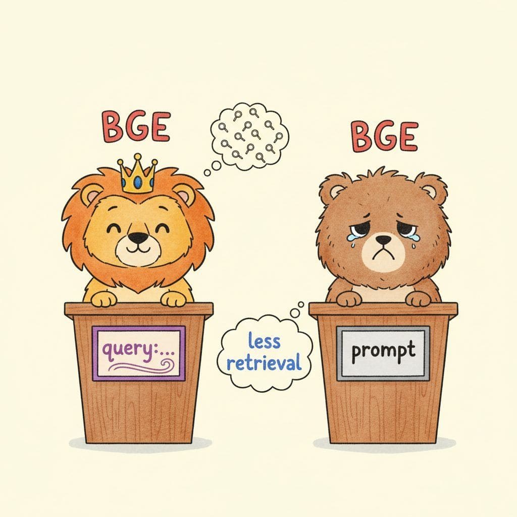
36.4.9 Domain-specific and niche embedders
General-purpose embedders score well on aggregate benchmarks but lose 5-15 points to domain-tuned alternatives on in-domain data. The 2026 domain-specific landscape:
- Code embedders: jina-embeddings-v2-code, UniXcoder, CodeT5+, and Voyage's voyage-code-3 are the canonical code-specific embedders. Pick when the corpus is source code; general embedders trained on prose underperform on identifiers and structured syntax.
- Biomedical embedders: PubMedBERT, BioBERT, SciBERT, and ClinicalBERT are the open-weight biomedical encoders. Pick when the corpus is PubMed-style biomedical literature; the gap to general embedders on biomedical retrieval can be 10+ NDCG points.
- Legal embedders: LegalBERT, LEGAL-BERT, and Voyage's voyage-law-2 are the legal-domain choices. Pick for case-law and contract corpora where legal-vocabulary depth matters.
- Financial embedders: FinBERT, Prosus FinBERT, and Voyage's voyage-finance-2 cover financial filings, earnings calls, and SEC documents. Pick when retrieving from financial-domain text.
- Multilingual focused embedders: multilingual-E5-large-instruct, BGE-multilingual-gemma2, and Cohere Embed v3 (multilingual variant) are stronger than English-trained models for non-English corpora. Pick when the corpus is genuinely multilingual.
The recurring 2024-25 finding: a domain-tuned 110M-parameter model often beats a general-purpose 7B model on in-domain retrieval. Domain fine-tuning is the highest-leverage upgrade once you have a working general-purpose baseline.
36.4.10 Fine-tuning your own embedder
If a domain-tuned model does not exist for your domain, fine-tuning your own is the next step. The 2026 standard recipe:
- Base model: start from a strong open-weights generalist (BGE-base, Stella, mxbai-embed, or one of the E5 series). For small budgets, BGE-base is the right starting point; for larger budgets, the 7B-class models (NV-Embed, Linq-Embed) give more headroom.
- Training objective: contrastive loss with hard negatives mined via the in-progress model (the ANCE recipe, Xiong et al. 2020). The sentence-transformers 3.x trainer plus the FlagEmbedding training code both implement this out of the box.
- Data: 10K to 100K query-positive pairs are usually enough for a meaningful improvement; below 1K, the fine-tune adds noise. Synthetic query generation via an LLM is the most common way to produce the pairs when human labels are unavailable.
- Hard negatives: mine 5-10 hard negatives per query from the top-100 retrieval results of the base model; filter out true positives via either human review or LLM-as-judge.
- Evaluation: hold out 10-20% of the pairs for evaluation; the headline metric is NDCG@10 on the held-out set. Cross-check against BEIR or MTEB to detect catastrophic forgetting.
- Compute: a single A100 fits a BGE-base fine-tune in 4-12 hours; a 7B model needs 8x A100 or 1x H100 and 1-3 days. Most fine-tunes finish in under a day on commodity cloud GPUs.
The expected improvement from a single fine-tune is 3-10 NDCG points on in-domain data versus the base model. Beyond that, the next leverage points are the reranker (which often gives another 2-5 points) and the retrieval pipeline structure (hybrid, query rewriting, contextual retrieval).
The training objective behind every BGE, E5, NV-Embed, Stella, Linq-Embed, and most closed-API embedders in 2026 is InfoNCE (Oord et al. 2018, "Representation Learning with Contrastive Predictive Coding"), applied at the query-passage pair level. For a query $q$ with a positive passage $d^+$ and a batch of negatives $\{d_1^-, \ldots, d_N^-\}$:
$$\mathcal{L}_{\text{InfoNCE}} = -\log \frac{\exp(s(q, d^+) / \tau)}{\exp(s(q, d^+) / \tau) + \sum_{i=1}^{N} \exp(s(q, d_i^-) / \tau)}$$
where $s(q, d) = q \cdot d / (\|q\| \|d\|)$ is cosine similarity (or scaled dot product) and $\tau$ is the temperature.
Temperature. Small $\tau$ (e.g. 0.01-0.05) sharpens the softmax, forcing the model to push negatives strongly away from the query; large $\tau$ (e.g. 0.5-1.0) softens it. The 2024-25 community default sits around $\tau = 0.02$ for English retrieval and $\tau = 0.05$ for multilingual where the negative distribution is noisier. Too-small $\tau$ collapses positives into delta functions and amplifies label noise; too-large $\tau$ fails to separate near-duplicates.
Hard negatives. Random in-batch negatives are easy (a typical document is trivially distinct from a query); the gradient signal saturates quickly. ANCE-style hard-negative mining (Xiong et al. 2020) refreshes negatives every few epochs from the current model's top-100 retrieval errors, where each negative is "almost right" by current parameters. The empirical recipe: 5-10 hard negatives per query, refreshed every 2-4 epochs, with a small fraction (1-2%) screened by LLM-judge to filter false negatives (documents that are actually relevant but unlabeled). This single step lifts MTEB scores by 3-7 points over random-negative baselines and is the single most important reason every BGE-family model outperforms naive DPR.
from sentence_transformers import SentenceTransformer, losses, InputExample
from sentence_transformers.trainer import SentenceTransformerTrainer
from sentence_transformers.training_args import SentenceTransformerTrainingArguments
from datasets import Dataset

# 1. Load a strong base model.
model = SentenceTransformer("BAAI/bge-base-en-v1.5")

# 2. Prepare training data: (query, positive, hard_neg_1, hard_neg_2, ...) tuples.
train_pairs = Dataset.from_list([
    {"anchor": q, "positive": p, "negative": n}
    for q, p, n in your_mined_triplets
])

# 3. Use a triplet loss with hard negatives.
loss = losses.MultipleNegativesRankingLoss(model)

# 4. Train.
trainer = SentenceTransformerTrainer(
    model=model, loss=loss, train_dataset=train_pairs,
    args=SentenceTransformerTrainingArguments(
        output_dir="bge-base-domain-finetuned",
        num_train_epochs=2, per_device_train_batch_size=64,
        learning_rate=2e-5, warmup_ratio=0.1,
    ),
)
trainer.train()
model.save_pretrained("bge-base-domain-finetuned")
The training step is 50 lines; the data preparation (mining hard negatives, filtering false negatives) is the part that takes a week. Budget 80% of the project time for the data, not the training loop.
What's Next?
In the next section, Section 36.5: External Reading and Communities, we build on the material covered here.