Why memorize a million rows when you can simply ask the database a well-formed question?
RAG, SQL-Fluent AI Agent
Most enterprise knowledge lives in databases, not documents. Sales figures, inventory counts, customer records, and financial data are stored in relational databases and spreadsheets. Text-to-SQL enables users to query these structured data sources using natural language, bridging the gap between business questions and database queries. Combined with traditional document-based RAG (as covered in Section 32.1), this creates hybrid retrieval systems that can answer questions requiring both factual context and precise numerical data.
Prerequisites
Text-to-SQL and structured-data RAG extend the retrieval paradigm from Section 32.1 to tabular and relational data sources. You should be comfortable with basic SQL concepts and understand how LLMs generate structured output, a topic introduced in Section 12.2. The evaluation challenges discussed here connect to the broader LLM evaluation framework covered later in the book.
32.4.1 LLMs and Tabular Data
Tables break LLMs in ways free-form text does not. Strict row-column structure, typed values, foreign keys, and uniqueness constraints all matter. Stuff a 50-row table into the context window and the model reasons over it directly. Bigger than that and you flip the problem: get the model to write SQL or pandas that pulls only what you need.
32.4.1.1 Direct Table Reasoning
For tables under 50 rows, drop them straight in the prompt. Markdown with clear column headers beats raw CSV: the model reads the schema visually. The approach breaks two ways at scale, the table overflows context, and LLM arithmetic across many rows is flaky. Beyond 50 rows, switch to query generation.
# Direct table Q&A: serialize a small DataFrame into the prompt and let the LLM
# answer questions about it. Works for tables under ~50 rows; bigger tables need text-to-SQL.
import pandas as pd
from openai import OpenAI
client = OpenAI()
def ask_about_table(df: pd.DataFrame, question: str):
    """Ask a question about a small DataFrame directly."""
    # Convert to markdown for clear formatting
    table_md = df.to_markdown(index=False)
    response = client.chat.completions.create(
        model="gpt-4o",
        messages=[{
        "role": "system",
        "content": "You are a data analyst. Answer questions about "
        "the provided table. Show your reasoning."
        }, {
        "role": "user",
        "content": f"Table:\n{table_md}\n\nQuestion: {question}"
        }]
    )
return response.choices[0].message.contentThe Spider benchmark for text-to-SQL contains 10,181 questions across 200 databases. State-of-the-art LLMs now score above 85% on it, which sounds impressive until you realize that the remaining 15% includes queries like nested correlated subqueries with HAVING clauses that most human SQL developers would also get wrong on the first try.
32.4.2 Text-to-SQL: Architecture
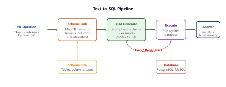
Text-to-SQL turns "show me last quarter's top customers" into a runnable query. The hard part is not the SQL grammar, it is picking the right tables, columns, and joins from a schema the user never names. Modern LLM pipelines crack 85% on Spider by stacking three tricks: schema linking, few-shot examples, and an execute-then-repair loop. Figure 32.4.1a traces the pipeline end to end.
The single highest-leverage improvement for text-to-SQL accuracy is including 3 to 5 diverse, annotated examples in the prompt (few-shot learning). Column descriptions and sample rows help, but well-chosen examples teach the model your schema's naming conventions, join patterns, and edge cases more effectively than any amount of schema documentation.
32.4.2.1 Schema Linking
Schema linking is the process of identifying which database tables and columns are relevant to the
user's question. This is often the hardest step because users rarely use exact column names. A user
asking about "revenue" might mean the total_amount column in the orders
table, or the annual_revenue column in the companies table.
A concrete failure: a user asks "show me churn last quarter." Your schema has no churn column, but it has users.last_active_date, users.cancellation_date, and subscriptions.status. The LLM needs to recognize that "churn" is a derived concept (users where cancellation_date BETWEEN Q3_start AND Q3_end, or status = 'cancelled' with a date filter). Without good schema linking, the model might invent a churn column (and the query fails on execution), or it might query the wrong table (and silently return the wrong number). The fix is including a few-shot example that demonstrates the canonical pattern for "churn" on your schema, plus a column description like cancellation_date - the date a user ended their subscription; used to compute churn rate.
# Pull table names, columns, and sample rows out of the database to feed the LLM.
# The richer the schema context, the more accurate the generated SQL.
def get_schema_context(db_connection, relevant_tables=None):
    """Extract schema information for the LLM prompt."""
    schema_parts = []
    # Get all tables or filter to relevant ones
    tables = relevant_tables or get_all_tables(db_connection)
    for table in tables:
        columns = get_columns(db_connection, table)
        col_info = []
        for col in columns:
            col_str = f" {col['name']} {col['type']}"
            if col.get("primary_key"):
                col_str += " PRIMARY KEY"
                if col.get("foreign_key"):
                    col_str += f" REFERENCES {col['foreign_key']}"
                    col_info.append(col_str)
                    # Include sample values for disambiguation
                    samples = get_sample_values(db_connection, table, limit=3)
                    schema_parts.append(
                        f"CREATE TABLE {table} (\n"
                        + ",\n".join(col_info)
                        + f"\n);\n-- Sample rows: {samples}"
                        )
return "\n\n".join(schema_parts)32.4.2.2 SQL Generation with Few-Shot Examples
Once the schema context is prepared, the next step is generating executable SQL from the user's natural language question. Code Fragment 32.4.3 below demonstrates how to combine schema information with optional few-shot examples in a single LLM call.
# Generate executable SQL from a natural-language question. Optional few-shot
# examples (question + expected SQL pairs) steer the model toward your SQL dialect.
def text_to_sql(question, schema_context, examples=None):
    """Generate SQL from natural language question."""
    few_shot = ""
    if examples:
        few_shot = "\n\nExamples:\n" + "\n".join([
            f"Q: {ex['question']}\nSQL: {ex['sql']}"
            for ex in examples
            ])
        response = client.chat.completions.create(
            model="gpt-4o",
            messages=[{
            "role": "system",
            "content": f"""You are a SQL expert. Generate a SQL query to
            answer the user's question based on this schema:
            {schema_context}
            {few_shot}
            Rules:
            - Use only tables and columns from the schema
            - Return ONLY the SQL query, no explanation
            - Use standard SQL compatible with PostgreSQL
            - Add LIMIT 100 to prevent unbounded results
            - Handle NULLs appropriately"""
            }, {
            "role": "user",
            "content": question
            }],
            temperature=0.0
            )
        sql = response.choices[0].message.content.strip()
        # Remove markdown code fences if present
        sql = sql.replace("```sql", "").replace("```", "").strip()
return sqlThe choice of few-shot examples dramatically affects text-to-SQL accuracy. The most effective strategy is to embed the user's question and retrieve the most similar examples from a curated example bank using vector similarity. This "dynamic few-shot" approach ensures that the examples shown to the LLM are maximally relevant to the current question, improving accuracy by 10 to 20% compared to fixed examples on complex queries.
32.4.3 Error Correction and Self-Healing Queries
Even the best LLMs generate incorrect SQL queries. Common errors include referencing nonexistent columns, incorrect join conditions, missing GROUP BY clauses, and type mismatches. A robust text-to-SQL pipeline includes an error correction loop that catches execution failures, sends the error message back to the LLM along with the original query, and asks for a corrected version.
# Self-correcting SQL loop: when the generated query throws, feed the error back
# to the LLM and ask for a fix. Bounded retries keep one bad query from looping forever.
import sqlite3
def execute_with_retry(question, schema_context, db_path,
    max_retries=3):
    """Execute SQL with automatic error correction."""
    conn = sqlite3.connect(db_path)
    error_history = []
    for attempt in range(max_retries):
        # Generate SQL (include errors from prior attempts)
        if error_history:
            error_context = "\n".join([
                f"Attempt {e['attempt']}: {e['sql']}\n"
                f"Error: {e['error']}"
                for e in error_history
                ])
            question_with_context = (
                f"{question}\n\nPrevious failed attempts:\n"
                f"{error_context}\n\nFix the errors."
                )
        else:
            question_with_context = question
            sql = text_to_sql(question_with_context, schema_context)
            try:
                cursor = conn.execute(sql)
                columns = [desc[0] for desc in cursor.description]
                rows = cursor.fetchall()
                return {
                    "sql": sql,
                    "columns": columns,
                    "rows": rows,
                    "attempts": attempt + 1
                    }
            except Exception as e:
                error_history.append({
                    "attempt": attempt + 1,
                    "sql": sql,
                    "error": str(e)
                    })
                return {"error": "Failed after max retries",
"history": error_history}Allowing an LLM to generate and execute SQL queries introduces serious security risks. Always enforce these safeguards: (1) use a read-only database connection (no INSERT, UPDATE, DELETE, or DROP), (2) set query timeouts to prevent long-running queries, (3) limit result set sizes, (4) validate generated SQL against an allowlist of permitted operations before execution, and (5) run queries against a replica or snapshot, never the production database directly.
32.4.4 Text-to-SQL Benchmarks
Standard benchmarks measure text-to-SQL system performance across databases of varying complexity. The two most widely used benchmarks are Spider and BIRD, which test different aspects of the text-to-SQL challenge.
| Benchmark | Databases | Questions | Key Challenge | SOTA Accuracy |
|---|---|---|---|---|
| Spider | 200 databases | 10,181 | Cross-database generalization | ~87% (execution) |
| BIRD | 95 databases | 12,751 | Real-world complexity, external knowledge | ~72% (execution) |
| WikiSQL | 26,521 tables | 80,654 | Single-table, simpler queries | ~93% (execution) |
| SParC | 200 databases | 4,298 | Multi-turn conversational SQL | ~70% (execution) |
Text-to-SQL is one of the rare LLM features that already has multiple production deployments. Snowflake Cortex Analyst (2024) and Databricks Genie (2024) both expose a natural-language-to-SQL interface inside the data warehouse, generating SQL against governed semantic models. AWS QuickSight Q and Google Cloud's Looker "Conversational Analytics" (2024) are the equivalents from hyperscaler BI platforms. On the startup side, Defog.ai's SQLCoder model (open weights) powers internal text-to-SQL at HSBC and several Fortune-500 finance teams. The accuracy gap between Spider (~87 percent) and BIRD (~72 percent) explains why every shipped product layers a confirmation step or a constrained schema: production text-to-SQL is best deployed as an "assist" feature, not as auto-execute.
32.4.5 CSV and Spreadsheet Processing
Not all structured data lives in databases. CSV files, Excel spreadsheets, and Google Sheets are ubiquitous in business environments. LLMs can process these by either loading them into an in-memory database (SQLite) for SQL queries or generating pandas code for direct manipulation.
# Load a CSV into an in-memory SQLite database so the LLM can hit it with
# SQL queries instead of doing brittle arithmetic across rows in the prompt.
import pandas as pd
import sqlite3
def csv_to_queryable(csv_path, table_name="data"):
    """Load a CSV into SQLite for text-to-SQL querying."""
    df = pd.read_csv(csv_path)
    # Create in-memory database
    conn = sqlite3.connect(":memory:")
    df.to_sql(table_name, conn, index=False)
    # Generate schema description
    schema = f"Table: {table_name}\nColumns:\n"
    for col in df.columns:
        dtype = str(df[col].dtype)
        sample = df[col].dropna().head(3).tolist()
        schema += f" {col} ({dtype}), e.g., {sample}\n"
        return conn, schema

# Usage
conn, schema = csv_to_queryable("sales_data.csv", "sales")
result = execute_with_retry(
    "What are the top 5 products by total revenue this quarter?",
    schema, conn
)32.4.6 Hybrid Structured/Unstructured Retrieval
Many real-world questions require combining structured data (from databases) with unstructured context (from documents). For example, "Why did Q3 revenue decline for our enterprise segment?" requires both the numerical revenue data from a database and contextual explanations from quarterly reports, meeting notes, or market analyses. Figure 32.4.2a shows how hybrid retrieval merges database results with document context.
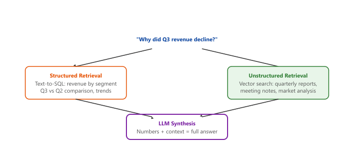
The most common pattern for hybrid retrieval is to route the question to both a text-to-SQL pipeline and a document RAG pipeline in parallel, then combine both result sets in the LLM prompt. The structured data provides the "what" (exact numbers, trends, comparisons), while the unstructured data provides the "why" (explanations, context, causal factors). This combination produces answers that are both precise and insightful.
32.4.7 Multi-Table Joins and Complex Queries
The hardest text-to-SQL queries involve multiple tables with complex join conditions, nested subqueries, window functions, and conditional aggregations. These queries require the LLM to understand the database's relational structure: which tables connect to which, through what foreign keys, and with what cardinality.
Three techniques significantly improve accuracy on complex multi-table queries: (1) Schema descriptions: annotating each column with a human-readable description of what it contains and how it relates to business concepts. (2) Join hints: explicitly listing common join patterns (e.g., "orders.customer_id joins to customers.id"). (3) Chain-of-thought SQL: asking the LLM to first write out its reasoning about which tables and joins are needed before generating the SQL, which reduces errors on queries requiring 3+ table joins.
Who: A data analytics team lead at a retail chain with 400 stores
Situation: Regional managers needed daily access to sales metrics (revenue by category, inventory levels, promotional performance) but had to submit requests to the analytics team because the BI dashboard was too rigid for ad-hoc questions.
Problem: The analytics team processed 60+ ad-hoc data requests per week, each taking 15 to 30 minutes. Managers often waited 2 days for answers, which made the data stale by the time they received it.
Dilemma: Giving managers direct SQL access was a security risk and required training they lacked. A fully natural-language interface risked generating incorrect queries that could produce misleading business decisions.
Decision: They built a text-to-SQL system with guardrails: the LLM generated read-only SELECT queries, a schema description layer exposed only pre-approved tables and columns, and every generated query was validated against a set of SQL safety rules before execution.
How: Table and column descriptions (with business-friendly names and sample values) were injected into the prompt. Ambiguous queries triggered a clarification step. Results were returned as formatted tables with a natural language summary explaining the numbers.
Result: Managers self-served 78% of their data questions. The analytics team's ad-hoc request volume dropped from 60 to 13 per week. Query accuracy (validated against analyst-written queries) was 91% on a test set of 200 common questions.
Lesson: Text-to-SQL works best when you constrain the schema surface area, enforce read-only access, and add a clarification step for ambiguous queries rather than guessing the user's intent.
32.4.8 Automated RAG Pipeline Optimization
Building a RAG pipeline involves dozens of configuration decisions: which embedding model to use, what chunk size and overlap to set, how many documents to retrieve, whether to apply reranking, what prompt template to use for generation, and how to handle multi-hop queries. Traditionally, teams tune these parameters manually through trial and error. Automated RAG optimization treats the entire pipeline as a configurable system and uses systematic search to find the best configuration for a given dataset and task. This approach is gaining traction as RAG matures from a research prototype into a production pattern.
32.4.8.1 RAG as a Configurable Pipeline
The key insight behind AutoRAG is that every RAG pipeline is a composition of interchangeable components, each with its own hyperparameters. Just as AutoML tunes model architecture and learning rate, AutoRAG tunes retrieval and generation parameters:
| Pipeline Stage | Configurable Parameters | Example Options |
|---|---|---|
| Chunking | Strategy, chunk size, overlap | Recursive (512 tokens, 10% overlap) vs. semantic chunking |
| Embedding | Model, dimensionality | OpenAI text-embedding-3-small vs. Cohere embed-v3 vs. BGE-M3 |
| Retrieval | Top-k, similarity metric, hybrid weights | Top-5 cosine vs. top-10 with BM25 hybrid (0.7/0.3 blend) |
| Reranking | Model, threshold | No reranking vs. Cohere rerank-v3 vs. cross-encoder |
| Generation | Model, temperature, prompt template | GPT-4o with structured prompt vs. Claude with concise template |
32.4.8.2 RAGAs: Evaluation Metrics for RAG
Meaningful optimization requires meaningful metrics. The RAGAs framework (Shahul et al., 2023) provides a suite of evaluation metrics specifically designed for RAG systems. These metrics evaluate both the retrieval and generation stages independently, enabling targeted optimization. The key metrics are:
- Context Precision: What fraction of retrieved passages are actually relevant to the question? High precision means the retriever is not wasting context window space on irrelevant documents.
- Context Recall: What fraction of the information needed to answer the question is present in the retrieved passages? High recall means the retriever is finding all the relevant evidence.
- Faithfulness: Is every claim in the generated answer supported by the retrieved context? This directly measures hallucination risk.
- Answer Relevancy: Does the generated answer actually address the question asked? A faithful answer can still be irrelevant if the model focuses on the wrong part of the context.
The ragas package (v0.2+, 2024 to 2026) ships every metric named above as a one-line evaluator that runs against a Hugging Face Dataset of (question, retrieved-contexts, answer, reference) rows. Pair it with a small golden set and run it in CI; the metrics live as floats you can chart over time, so a regression in faithfulness becomes a failing build instead of a Slack thread.
Show code
pip install ragas datasets
from datasets import Dataset
from ragas import evaluate
from ragas.metrics import (
    LLMContextRecall, Faithfulness, ContextPrecision, ResponseRelevancy,
)

ds = Dataset.from_list([
    {
        "user_input": "What is our vacation policy?",
        "retrieved_contexts": ["Full-time employees receive 20 days of paid vacation."],
        "response": "Full-time employees receive 20 paid vacation days per year.",
        "reference": "20 paid vacation days annually for full-time employees.",
    },
])
report = evaluate(
    ds,
    metrics=[LLMContextRecall(), Faithfulness(), ContextPrecision(), ResponseRelevancy()],
)
print(report.to_pandas()) # one row per example with per-metric scoresevaluate() call.RAGAS is the best-known framework, but it is not the only one. Three alternatives are worth naming because each occupies a slightly different niche in production stacks.
- ARES (Saad-Falcon et al., NAACL 2024) trains a lightweight judge model on synthetic in-domain examples and then evaluates context relevance, answer faithfulness, and answer relevance with that fine-tuned judge instead of calling a frontier LLM per query. The trade-off versus RAGAS is upfront fine-tuning cost in exchange for lower per-evaluation cost and tighter domain alignment; ARES is a good fit when the eval set is large enough that the judge-API bill itself becomes the bottleneck.
- TruLens (TruEra) is the team that coined the "RAG triad" terminology (context relevance, groundedness, answer relevance) reused above and in Section 32.2.2. TruLens packages those three metrics as runtime feedback functions and an observability dashboard, so each production query gets a score tile next to the trace; it sits closer to APM than to a CI metric library.
- DeepEval (Confident AI) presents RAG metrics with a pytest-style API (
assert_test,@pytest.mark.deepeval), which is convenient when the team already runs pytest in CI; see the library-shortcut callout in Section 36.2.
TruLens wraps any LangChain or LlamaIndex chain and emits the RAG triad (context relevance, groundedness, answer relevance) per call to a local SQLite store; a built-in dashboard surfaces the lowest-scoring traces for review.
from trulens.core import TruSession, Feedback
from trulens.providers.openai import OpenAI as TruOpenAI
from trulens.apps.langchain import TruChain

provider = TruOpenAI()
session = TruSession()

f_groundedness   = Feedback(provider.groundedness_measure_with_cot_reasons).on_input_output()
f_context_rel    = Feedback(provider.context_relevance).on_input_output()
f_answer_rel     = Feedback(provider.relevance).on_input_output()

tru_chain = TruChain(
    rag_chain,
    app_id="rag-prod",
    feedbacks=[f_groundedness, f_context_rel, f_answer_rel],
)
with tru_chain as recording:
    rag_chain.invoke("What is our vacation policy?")
session.get_records_and_feedback()[0].head()32.4.8.3 Manual vs. Automated RAG Tuning
| Dimension | Manual Tuning | Automated (AutoRAG) |
|---|---|---|
| Configuration space explored | 3 to 5 configurations | 50 to 200+ configurations |
| Time investment | Days to weeks | Hours (automated evaluation) |
| Reproducibility | Low (undocumented decisions) | High (logged experiments, metric history) |
| Discovery of non-obvious configs | Unlikely | Common (e.g., small chunks + reranker beats large chunks) |
| Upfront cost | Low (human time) | Moderate (compute for eval runs) |
| Best for | Prototypes, simple pipelines | Production systems, complex multi-stage pipelines |
The most important lesson from AutoRAG research is that optimal configurations are often counterintuitive. Teams frequently discover that smaller chunk sizes with aggressive reranking outperform larger chunks without reranking, or that a cheaper embedding model paired with a cross-encoder reranker beats a premium embedding model used alone. Without systematic evaluation across many configurations, these non-obvious tradeoffs remain hidden. The chunking evaluation framework from Section 31.6 and the LLM-as-judge evaluation pattern from Section 42.2 provide the building blocks for automated RAG evaluation.
Who: A platform team managing a customer support knowledge base for a B2B SaaS vendor.
Situation: The team owned 50,000 articles and a RAG pipeline that had been hand-tuned over two weeks to 72% answer accuracy as judged by support agents.
Problem: Further manual tuning had plateaued, and each change required a fresh round of agent grading; the configuration surface (chunk size, embedding model, retrieval strategy, reranking, generation model) was too large to explore by hand.
Dilemma: Either accept the 72% plateau and ship, or invest engineering time in an automated search whose payoff was uncertain.
Decision: They built an automated evaluation harness with 200 ground-truth question-answer pairs and let it search a 96-configuration grid.
How: The harness used RAGAs metrics (faithfulness, context precision, answer relevancy) and tested 96 configurations: 4 chunk sizes (256, 512, 768, 1024 tokens), 3 embedding models, 2 retrieval strategies (dense-only vs. hybrid), 2 reranking options (none vs. cross-encoder), and 2 generation models.
Result: The winning configuration (384-token chunks with Cohere embed-v3, hybrid retrieval, cross-encoder reranking, and GPT-4o-mini for generation) achieved 86% answer accuracy, a 14-point improvement. Notably, this configuration used a cheaper generation model than the manually tuned version, reducing per-query cost by 40% while improving quality.
Lesson: Automated configuration search routinely beats hand-tuning on RAG pipelines because the optimum is often counterintuitive, and the search cost is dwarfed by the lifetime savings from a better configuration.
For the canonical RAG evaluation triangle (retrieval recall, faithfulness, end-to-end correctness) that text-to-SQL pipelines also need, see Section 43.1: RAG Evaluation. For when to push the text-to-SQL accuracy ceiling via fine-tuning rather than prompting, see Section 16.1: When and Why to Fine-Tune. For the structured-output techniques that keep generated SQL parseable, see Section 11.2: Structured Output.
LLM-native SQL generation is improving through specialized fine-tuning on SQL benchmarks (BIRD, Spider 2.0), with models like SQLCoder and DIN-SQL achieving near-human accuracy on complex queries. Semantic layers (e.g., Cube, dbt Metrics) provide a business-friendly abstraction over raw database schemas, reducing hallucinated column names and join errors. Multi-turn SQL conversations allow users to iteratively refine queries through natural language, with the system maintaining query history and context. Research into privacy-preserving text-to-SQL is developing methods to generate accurate queries without exposing raw data to the LLM. AutoRAG frameworks (AutoRAG, Ragas, ARES) are systematizing RAG pipeline optimization by combining automated evaluation with configuration search, paralleling the evolution of hyperparameter tuning in traditional ML.
- Text-to-SQL unlocks database-backed RAG: By converting natural language to SQL, LLMs can query relational databases for precise numerical answers that vector search cannot provide.
- Schema linking is the critical bottleneck: Correctly mapping user terms to database columns determines success; enhance it with column descriptions, sample values, and dynamic few-shot examples.
- Error correction loops are essential: Automatic retry with error feedback catches most SQL generation mistakes, improving reliability from roughly 70% to over 85% on complex queries.
- Security is non-negotiable: Read-only connections, query timeouts, result limits, SQL validation, and database replicas are mandatory safeguards for any production text-to-SQL system.
- Hybrid retrieval combines precision and context: The most powerful answers come from combining structured data (exact numbers) with unstructured context (explanations), retrieved in parallel and synthesized by the LLM.
Show Answer
Show Answer
Show Answer
Show Answer
Show Answer
Exercises
Why is it useful to have an LLM generate SQL queries rather than building a custom search interface? What risks does this introduce?
Show Answer
Text-to-SQL lets non-technical users query databases using natural language, eliminating the need to learn SQL. Risks: SQL injection if queries are executed without sandboxing, incorrect queries that return wrong data with high confidence, and queries that are too expensive (full table scans, cross-joins).
Explain what schema linking is and why it is the most critical step in a text-to-SQL pipeline. What happens when schema linking fails?
Show Answer
Schema linking maps natural language terms to table and column names. Without it, the LLM may reference non-existent columns or join the wrong tables. Failure produces syntactically valid but semantically incorrect SQL.
Describe how error correction works in a text-to-SQL system. Why is it better to have the LLM fix its own SQL than to simply retry?
Show Answer
The LLM receives the SQL error message (e.g., "column 'user_name' not found") and the original query, allowing it to correct the specific mistake. Blind retries would generate the same error. Self-correction works because the error message provides targeted feedback.
A user asks "How did our top customers perform last quarter?" This requires both a database query (customer metrics) and document retrieval (qualitative analysis). How would you design a system that handles both?
Show Answer
Use a query router that classifies the intent: (a) structured/quantitative questions go to text-to-SQL, (b) qualitative/descriptive questions go to vector retrieval, (c) hybrid questions invoke both and combine results in the final prompt.
Explain the concept of automated RAG pipeline optimization. What components are tuned, and what metrics guide the search?
Show Answer
AutoRAG treats the RAG pipeline configuration as a hyperparameter optimization problem. Components tuned: chunk size, overlap, embedding model, retrieval top-K, reranker, prompt template. Metrics: answer correctness (LLM-as-judge), faithfulness (grounded in sources), retrieval recall, latency, and cost.
Create a SQLite database with 3 tables. Write a prompt that provides the schema to an LLM and ask it to generate SQL for 5 natural language questions. Execute the SQL and check correctness.
Extend your text-to-SQL pipeline with error handling: if the generated SQL fails, send the error message back to the LLM and ask it to fix the query. Allow up to 3 retries.
Build a pipeline that takes a CSV file, infers the schema, converts it to a SQLite database, and answers natural language questions about the data using text-to-SQL.
Implement a simple AutoRAG optimization: for a fixed test set of 20 questions, sweep over chunk sizes (128, 256, 512), top-K values (3, 5, 10), and with/without reranking. Report the best configuration based on answer accuracy.
What Comes Next
In the next section, Section 35.6: RAG Frameworks & Orchestration, we survey RAG frameworks and orchestration tools, the practical libraries that simplify building production RAG systems.