"My classifier achieves 99% accuracy. Unfortunately, 99% of my data belongs to one class. Time to learn about focal loss."
Finetune, Class-Imbalanced AI Agent
Classification is the most common fine-tuning task in production NLP. Sentiment analysis, spam detection, intent classification, named entity recognition, and content moderation all reduce to some form of classification. Training data for these classifiers can be generated efficiently using LLM-assisted labeling. This approach is common in hybrid ML and LLM systems where a small, fast classifier handles high-volume tasks. The approach is different from generative fine-tuning (SFT): instead of training the model to generate text, you add a classification head on top of the pretrained model and train it to predict discrete labels. Hugging Face's AutoModel classes make this straightforward, but there are important decisions around architecture, loss functions, and class imbalance that determine whether your classifier works well in practice. The ML classification fundamentals from Section 0.1 provide the evaluation metrics and baseline approaches to compare against.
Prerequisites
Before starting, make sure you are familiar with fine-tuning basics as covered in Section 16.1: When and Why to Fine-Tune.
16.6.1 Classification Head Architecture
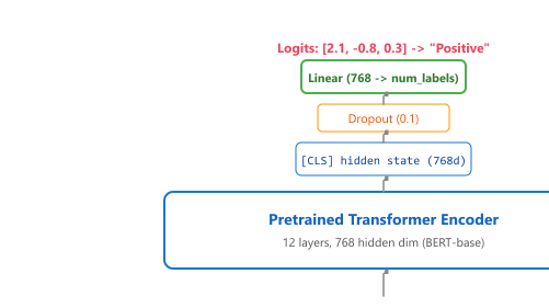
When fine-tuning a Transformer architecture for classification, you keep the pretrained encoder body and add a small classification head on top. The head is typically a linear layer (or a small MLP) that maps the model's hidden representation to class logits. The entire model (encoder plus head) is trained end-to-end, but the head learns from scratch while the encoder benefits from pretrained knowledge. Figure 16.6.1 illustrates this architecture.
For classification tasks with severe class imbalance (fewer than 5% of examples in the minority class), use focal loss instead of standard cross-entropy. Focal loss down-weights the contribution of easy, well-classified examples and focuses training on the hard cases. In practice, switching from cross-entropy to focal loss often improves minority-class F1 by 10 to 20 percentage points with no other changes to the training setup.
16.6.2 Single-Label Classification
Single-label classification is the simplest case: each input belongs to exactly one class. Examples include sentiment analysis (positive/negative/neutral), intent classification (booking/cancellation/inquiry), and content moderation (safe/unsafe). Hugging Face provides AutoModelForSequenceClassification that handles the architecture automatically.
Mental Model: The Attachment Head. Think of adding a classification head as attaching a specialized tool to a Swiss Army knife. The base model (the knife body) contains general-purpose language understanding in its hidden layers. The classification head (the attached tool) is a small linear layer that reads the model's internal representation and maps it to task-specific labels. During fine-tuning, you train both the attachment and (optionally) adjust the knife body itself, so the two work together seamlessly. Code Fragment 16.6.4 shows this approach in practice.
Code Fragment 16.6.2 defines training hyperparameters.
# Configure Hugging Face Trainer with training arguments
# Set learning rate schedule, batch size, and evaluation strategy
from transformers import (
    AutoModelForSequenceClassification,
    AutoTokenizer,
    TrainingArguments,
    Trainer,
    )
from datasets import load_dataset
import numpy as np
from sklearn.metrics import accuracy_score, f1_score, classification_report
# Load model with classification head
model_name = "bert-base-uncased"
num_labels = 3 # positive, negative, neutral
tokenizer = AutoTokenizer.from_pretrained(model_name)
model = AutoModelForSequenceClassification.from_pretrained(
    model_name,
    num_labels=num_labels,
    problem_type="single_label_classification",
    # Map label indices to human-readable names
    id2label={0: "negative", 1: "neutral", 2: "positive"},
    label2id={"negative": 0, "neutral": 1, "positive": 2},
    )
# Load and tokenize dataset
dataset = load_dataset("sst2") # Stanford Sentiment Treebank
def tokenize_function(examples):
    return tokenizer(
        examples["sentence"],
        padding="max_length",
        truncation=True,
        max_length=128,
        )
tokenized = dataset.map(tokenize_function, batched=True)
    # Define metrics
def compute_metrics(eval_pred):
    logits, labels = eval_pred
    predictions = np.argmax(logits, axis=-1)
    return {
        "accuracy": accuracy_score(labels, predictions),
        "f1_macro": f1_score(labels, predictions, average="macro"),
        "f1_weighted": f1_score(labels, predictions, average="weighted"),
        }
# Training configuration
training_args = TrainingArguments(
    output_dir="./checkpoints/sentiment-bert",
    num_train_epochs=3,
    per_device_train_batch_size=32,
    per_device_eval_batch_size=64,
    learning_rate=2e-5,
    weight_decay=0.01,
    warmup_ratio=0.1,
    eval_strategy="epoch",
    save_strategy="epoch",
    load_best_model_at_end=True,
    metric_for_best_model="f1_macro",
    report_to="wandb",
    )
trainer = Trainer(
    model=model,
    args=training_args,
    train_dataset=tokenized["train"],
    eval_dataset=tokenized["validation"],
    compute_metrics=compute_metrics,
    )
trainer.train()Code Fragment 16.6.4a loads the dataset.
# Load a pre-trained model for sequence classification fine-tuning
# The classification head is initialized randomly on top of the base model
from transformers import AutoModelForTokenClassification, AutoTokenizer
from datasets import load_dataset
# NER label scheme (BIO format)
label_list = [
    "O", "B-PER", "I-PER", "B-ORG", "I-ORG",
    "B-LOC", "I-LOC", "B-MISC", "I-MISC"
    ]
label2id = {l: i for i, l in enumerate(label_list)}
id2label = {i: l for i, l in enumerate(label_list)}
# Load model for token classification
model = AutoModelForTokenClassification.from_pretrained(
    "bert-base-uncased",
    num_labels=len(label_list),
    id2label=id2label,
    label2id=label2id,
    )
tokenizer = AutoTokenizer.from_pretrained("bert-base-uncased")
# Load CoNLL-2003 NER dataset
dataset = load_dataset("conll2003")
def tokenize_and_align_labels(examples):
    """Tokenize and align NER labels with subword tokens."""
    tokenized = tokenizer(
        examples["tokens"],
        truncation=True,
        is_split_into_words=True, # Input is already tokenized
        padding="max_length",
        max_length=128,
        )
    labels = []
    for i, label_ids in enumerate(examples["ner_tags"]):
        word_ids = tokenized.word_ids(batch_index=i)
        label_row = []
        previous_word_id = None
        for word_id in word_ids:
            if word_id is None:
                # Special tokens ([CLS], [SEP], [PAD])
                label_row.append(-100)
            elif word_id != previous_word_id:
                # First subword token of a word: use the word's label
                label_row.append(label_ids[word_id])
            else:
                # Subsequent subword tokens: use I- tag or -100
                original_label = label_ids[word_id]
                # Convert B- to I- for continuation tokens
                label_name = label_list[original_label]
                if label_name.startswith("B-"):
                    i_label = label_name.replace("B-", "I-")
                    label_row.append(label2id.get(i_label, original_label))
                else:
                    label_row.append(original_label)
                    previous_word_id = word_id
                    labels.append(label_row)
                    tokenized["labels"] = labels
                    return tokenized
tokenized_dataset = dataset.map(tokenize_and_align_labels, batched=True)Subword tokenization breaks word boundaries. A critical challenge in token classification is that the tokenizer may split a single word into multiple subword tokens. The word "Mountain" might become ["Mount", "##ain"]. You must carefully align the original word-level labels with the subword tokens. The standard approach is to assign the label to the first subword and use -100 (ignore) or the corresponding I- tag for continuation subwords.
16.6.3 Token Classification and Named Entity Recognition
Named Entity Recognition (NER) is the canonical token-level classification task: instead of one label per input, the model emits one label per token. NER tags spans like person names, organizations, locations, dates, and money amounts in text. The architecture mirrors single-label classification but with one critical change: the classification head is applied to every token's hidden state, not just the [CLS] token. Hugging Face provides AutoModelForTokenClassification as the drop-in counterpart of AutoModelForSequenceClassification.
16.6.3.1 CoNLL-2003 and BIO Tagging
The reference NER dataset is CoNLL-2003, an English newswire corpus annotated with four entity types: PER (person), ORG (organization), LOC (location), and MISC (miscellaneous). Tags follow the BIO scheme (sometimes BILOU): B-PER marks the beginning of a person span, I-PER marks the inside (continuation) of the same span, and O marks tokens outside any entity. With four entity types, the label set is $2 \times 4 + 1 = 9$ classes. The BIO scheme matters because it lets the model express that two adjacent person tokens (B-PER I-PER) form a single span ("John Smith") while two adjacent person tokens marked B-PER B-PER would be two separate one-word people ("John Mary").
16.6.3.2 Word-to-Subword Label Inheritance
NER annotations are defined at the word level, but transformer tokenizers operate at the subword level. The token "Washington" might split into ["Wash", "##ington"]; a single label has to be distributed across two tokens. The standard recipe is:
- Assign the original word label (e.g.,
B-LOC) to the first subword. - For every continuation subword, either repeat the corresponding
I-tag (e.g.,I-LOC) or assign the sentinel value-100, which PyTorch's cross-entropy loss skips entirely. - Always assign
-100to special tokens ([CLS],[SEP],[PAD]) so they do not contribute to the loss.
The HuggingFace tokenizer exposes word_ids() on its encoded output, returning a list that maps each subword position back to its source word index (with None for special tokens). The full alignment code is the tokenize_and_align_labels helper shown in Code Fragment 16.6.2b above. Skipping this step is the most common source of "my NER model trains but predicts garbage" bug reports.
16.6.3.3 seqeval: Entity-Level Evaluation
NER metrics must be computed at the entity level, not the token level. A prediction that gets two of three tokens correct in a three-token entity is a wrong entity prediction; the entire span must match. The seqeval library (one pip install) handles this correctly and is the standard reporting tool. Token-level F1 inflates scores because most tokens are O (outside-any-entity) and any model that predicts O everywhere will look respectable. Entity-level F1, by contrast, only rewards exact span matches and is the metric every CoNLL-style leaderboard expects.
If two systems both report "NER F1 = 0.92", they may be measuring different things. Always specify entity-level F1 (computed by seqeval) when comparing NER models. Token-level F1 on CoNLL-2003 is typically 5 to 10 points higher than the entity-level metric, so the two numbers are not interchangeable. The seqeval default uses the strict CoNLL evaluation script, which only credits an entity prediction when both the span boundaries and the type match exactly.
# Entity-level NER metrics with seqeval
# pip install seqeval evaluate
from seqeval.metrics import classification_report, f1_score
import numpy as np

def compute_ner_metrics(eval_pred, label_list):
    predictions, labels = eval_pred
    predictions = np.argmax(predictions, axis=2)

    # Drop -100 positions (special tokens, continuation subwords)
    true_labels = [
        [label_list[l] for l in seq if l != -100]
        for seq in labels
    ]
    pred_labels = [
        [label_list[p] for p, l in zip(pred_seq, label_seq) if l != -100]
        for pred_seq, label_seq in zip(predictions, labels)
    ]
    return {
        "entity_f1": f1_score(true_labels, pred_labels),
        "report": classification_report(true_labels, pred_labels, digits=3),
    }
Trainer. The compute_metrics function strips out the -100 positions (continuation subwords and special tokens) before calling seqeval, which expects clean per-word label sequences.16.6.4b SetFit: Few-Shot Classification Without Prompts
SetFit (Tunstall et al., 2022) is the production-default few-shot text-classification recipe and the one that should appear in every team's "I only have 8 labeled examples per class" playbook. The trick is to outsource the heavy lifting to an existing sentence-transformer.
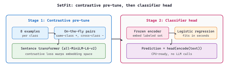
SetFit runs in two stages:
- Contrastive fine-tuning of a sentence transformer. Take a pretrained sentence-transformer (e.g.,
all-MiniLM-L6-v2) and a tiny labeled set (8 to 64 examples per class). Generate contrastive pairs on the fly: sentences from the same class form positives, sentences from different classes form negatives. The number of pairs grows quadratically in the number of examples, so even 8 examples per class produces thousands of training pairs. Fine-tune the sentence transformer on these pairs with a contrastive loss for a few epochs. The embedding space is now warped so that same-class sentences cluster together. - Train a classifier head on the embeddings. Encode every labeled example with the fine-tuned sentence transformer, then fit a vanilla classifier (logistic regression by default) on those embeddings. The head trains in seconds because logistic regression on a few hundred 384-dim vectors is trivial.
The result is competitive with full BERT fine-tuning on standard few-shot benchmarks while using zero prompts, zero generative model calls, no LLM API costs at inference, and a model small enough to deploy on a CPU. SetFit is what to reach for when the labeled dataset is too small for a normal fine-tune but too important to leave to a few-shot prompt. Figure 16.6.2 separates the two stages visually so the contrastive warp-up and the head-fit step do not blur together.
Code Fragment 16.6.4a is the smallest SetFit invocation that ships: one model, one trainer, one call to train.
# SetFit in its smallest possible form: two-stage few-shot text classification.
from setfit import SetFitModel, SetFitTrainer
from datasets import Dataset

train_dataset = Dataset.from_dict({
    "text": ["loved the support", "worst flight ever", "fast and friendly", "lost my luggage"],
    "label": [1, 0, 1, 0],
})
model = SetFitModel.from_pretrained("sentence-transformers/all-MiniLM-L6-v2")
trainer = SetFitTrainer(model=model, train_dataset=train_dataset, num_iterations=20)
trainer.train()
print(model.predict(["the staff were wonderful"]))
Code Fragment 16.6.4b: Minimal SetFit recipe. num_iterations=20 drives the on-the-fly pair generation that produces thousands of contrastive pairs from a handful of labels; the logistic head fits automatically inside trainer.train().
Concretely, stage one minimizes a contrastive distance loss over on-the-fly pairs $(x_i, x_j)$ with label $y_{ij} \in \{0, 1\}$ (1 if same class, 0 otherwise):
$$ \begin{aligned} \mathcal{L}_{\text{SetFit}} \;=\; \frac{1}{|\mathcal{P}|} \sum_{(x_i, x_j) \in \mathcal{P}} \Big[\; & y_{ij}\, d(f(x_i), f(x_j))^2 \;+\; \\ & (1 - y_{ij})\, \max\!\big(0,\; m - d(f(x_i), f(x_j))\big)^2 \;\Big] \end{aligned} $$
where $f$ is the sentence transformer, $d$ is Euclidean (or cosine) distance, and $m$ is a margin (default $0.5$). Same-class pairs pull together; different-class pairs are pushed at least $m$ apart. Stage two is a vanilla logistic regression head on the resulting embeddings, with the usual cross-entropy loss.
Suppose a 3-class sentiment task has $K = 8$ labeled examples per class, so $3K = 24$ examples total. SetFit generates contrastive pairs by sampling positive pairs from the same class and negative pairs across classes. With $K = 8$, each class yields $\binom{8}{2} = 28$ unique same-class pairs, so 3 classes produce $84$ positive pairs. The set of distinct cross-class pairs is $3 \cdot K \cdot K \cdot (3 - 1)/2 = 192$. With num_iterations=20, SetFit resamples and rebalances each epoch, yielding roughly $20 \cdot (84 + 192) \approx 5{,}500$ training pairs from the original 24 examples. That is the quadratic pair-generation trick: the labeled budget is fixed, but the contrastive signal grows with $K^2$.
Show code
# pip install setfit
from setfit import SetFitModel, SetFitTrainer
from datasets import Dataset

# 8 labeled examples per class is enough to start
train_ds = Dataset.from_dict({
    "text": ["Order arrived broken", "Great product!", "Late delivery", "Loved it!"],
    "label": [0, 1, 0, 1],  # 0=complaint, 1=praise
})
test_ds = Dataset.from_dict({"text": ["Worst experience ever", "Five stars"], "label": [0, 1]})

model = SetFitModel.from_pretrained("sentence-transformers/all-MiniLM-L6-v2")
trainer = SetFitTrainer(
    model=model,
    train_dataset=train_ds,
    eval_dataset=test_ds,
    num_iterations=20,           # pair-generation iterations
    num_epochs=1,
)
trainer.train()
print(trainer.evaluate())
print(model.predict(["Box arrived crushed"]))
SetFitTrainer.train(). The model trains in minutes on CPU and ships at sentence-transformer speed.If labeled examples per class are in the single digits and inference latency matters, SetFit usually wins on the cost-quality frontier. If labeled examples are in the hundreds per class and the task involves multi-step reasoning, full classifier-head fine-tuning (Section 16.6.2) or even an instruction-tuned LLM with few-shot prompts will do better. The rule of thumb is: under 32 examples per class, try SetFit first.
16.6.4 Sequence-Pair Tasks
Some classification tasks require comparing two input texts. Natural language inference (NLI) classifies the relationship between a premise and hypothesis as entailment, contradiction, or neutral. Semantic textual similarity (STS) scores the similarity between two sentences. Question answering classification determines whether a passage contains the answer to a question. All of these are handled with the same AutoModelForSequenceClassification by providing both texts to the tokenizer. Code Fragment 16.6.2d shows this approach in practice.
# Sequence pair classification (NLI example)
from transformers import AutoModelForSequenceClassification, AutoTokenizer
model = AutoModelForSequenceClassification.from_pretrained(
    "bert-base-uncased",
    num_labels=3,
    id2label={0: "entailment", 1: "neutral", 2: "contradiction"},
    label2id={"entailment": 0, "neutral": 1, "contradiction": 2},
)
tokenizer = AutoTokenizer.from_pretrained("bert-base-uncased")
# Tokenize a sentence pair
def tokenize_nli(examples):
    """Tokenize premise-hypothesis pairs."""
    return tokenizer(
        examples["premise"],
        examples["hypothesis"],
        padding="max_length",
        truncation=True,
        max_length=256,
    )
# The tokenizer automatically adds [SEP] between the two inputs:
# [CLS] premise tokens [SEP] hypothesis tokens [SEP]
sample = tokenizer(
    "A man is playing guitar on stage.",
    "A musician is performing live.",
    return_tensors="pt",
)
print(f"Input: {tokenizer.decode(sample['input_ids'][0])}")
print(f"Token type IDs: {sample['token_type_ids'][0][:20].tolist()}")
# token_type_ids: 0 for premise tokens, 1 for hypothesis tokens16.6.5 Handling Class Imbalance
Real-world classification datasets are almost always imbalanced. Fraud detection might have 0.1% positive examples; medical diagnosis datasets often have rare conditions representing less than 1% of cases. Without mitigation, the model will learn to predict the majority class and ignore rare but important classes.
| Strategy | How It Works | When to Use |
|---|---|---|
| Weighted loss | Assign higher loss weight to minority classes | Moderate imbalance (5:1 to 20:1) |
| Oversampling | Duplicate minority class examples | Small datasets where more data helps |
| Undersampling | Remove majority class examples | Very large datasets with extreme imbalance |
| Focal loss | Down-weight easy examples, focus on hard ones | Extreme imbalance (100:1+) |
| Synthetic data | Generate additional minority examples with LLMs | When real minority data is scarce |
Code Fragment 16.6.2e demonstrates this approach.
from transformers import Trainer
# Implement class-weighted loss for imbalanced dataset fine-tuning
# Minority classes receive higher loss weights to counteract skew
import torch
import torch.nn as nn
from torch.utils.data import WeightedRandomSampler
import numpy as np
class WeightedTrainer(Trainer):
    """Custom Trainer with class-weighted loss for imbalanced data."""
    def __init__(self, class_weights=None, **kwargs):
        super().__init__(**kwargs)
        if class_weights is not None:
            self.class_weights = torch.tensor(
                class_weights, dtype=torch.float32
                )
        else:
            self.class_weights = None
    def compute_loss(self, model, inputs, return_outputs=False, **kwargs):
        labels = inputs.pop("labels")
        outputs = model(**inputs)
        logits = outputs.logits
        if self.class_weights is not None:
            weight = self.class_weights.to(logits.device)
            loss_fn = nn.CrossEntropyLoss(weight=weight)
        else:
            loss_fn = nn.CrossEntropyLoss()
            loss = loss_fn(logits.view(-1, self.model.config.num_labels), labels.view(-1))
            return (loss, outputs) if return_outputs else loss
        # Calculate class weights from data distribution
    def compute_class_weights(labels: list, strategy: str = "inverse") -> list:
        """Compute class weights for imbalanced datasets."""
        unique, counts = np.unique(labels, return_counts=True)
        total = len(labels)
        if strategy == "inverse":
            # Weight inversely proportional to frequency
            weights = total / (len(unique) * counts)
        elif strategy == "sqrt_inverse":
            # Softer version: square root of inverse frequency
            weights = np.sqrt(total / (len(unique) * counts))
        elif strategy == "effective":
            # Effective number of samples (Class-Balanced Loss)
            beta = 0.9999
            effective_num = 1.0 - np.power(beta, counts)
            weights = (1.0 - beta) / effective_num
            # Normalize so mean weight = 1
            weights = weights / weights.mean()
            return weights.tolist()
        # Example: imbalanced dataset
        labels = [0]*9000 + [1]*800 + [2]*200 # 90% / 8% / 2% distribution
        weights = compute_class_weights(labels, strategy="sqrt_inverse")
        print(f"Class weights: {[f'{w:.2f}' for w in weights]}")
        print(f"Class 0 (90%): {weights[0]:.2f}x")
        print(f"Class 2 (2%): {weights[2]:.2f}x")
Use F1 macro (not accuracy) for imbalanced datasets. Accuracy is misleading when classes are imbalanced: a model that always predicts the majority class achieves 90% accuracy on a 90/10 split. F1 macro averages the F1 score across all classes equally, giving equal weight to minority classes. Always track per-class precision and recall to understand where the model is failing.
Adding a classification head to a pretrained transformer is like putting a sorting hat on a very well-read student. The model already understands the text; the head just needs to learn which bucket each understanding belongs in.
Why this matters: Classification fine-tuning is one of the most cost-effective uses of LLMs in production. A fine-tuned classifier model (even a small one like DeBERTa with 300M parameters) typically outperforms few-shot prompting of much larger models while being 100x cheaper to serve. This is the core tradeoff explored in the hybrid ML/LLM architectures of Chapter 14: use specialized fine-tuned models for well-defined classification tasks, and reserve large LLMs for tasks requiring open-ended generation.
Who: A compliance engineering team at a financial services company that needed to automatically tag internal documents with applicable regulatory frameworks (SOX, GDPR, PCI-DSS, HIPAA, CCPA, Basel III, and 15 others).
Situation: Each document could be tagged with multiple regulations (average of 2.3 tags per document). The team had 8,000 documents labeled by compliance officers, split across 21 regulatory categories with highly imbalanced distribution (GDPR appeared in 40% of documents, Basel III in only 3%).
Problem: An initial BERT-base classifier achieved 82% micro-F1 but only 54% macro-F1, performing poorly on rare categories. The compliance team required at least 75% macro-F1 because missing a regulatory tag could result in audit failures.
Dilemma: They could collect more training data for rare categories (expensive, slow), use data augmentation (limited effectiveness for specialized regulatory text), or address the imbalance through loss function modifications and training strategy changes.
Decision: They switched from standard binary cross-entropy to focal loss (reducing the contribution of easy, well-represented categories), added class-weighted sampling, and expanded the training set for the 5 rarest categories by 200 examples each using GPT-4 to generate synthetic regulatory documents reviewed by a compliance officer.
How: They used AutoModelForSequenceClassification with problem_type="multi_label_classification", replaced the default loss with focal loss (gamma=2.0), and implemented a custom sampler that oversampled rare categories by 3x. The synthetic data generation cost $180 in API fees plus 8 hours of compliance officer review time.
Result: Macro-F1 improved from 54% to 79%, exceeding the 75% threshold. Micro-F1 remained stable at 83%. The biggest gains came from rare categories: Basel III F1 rose from 31% to 72%, and HIPAA rose from 45% to 78%. Total compute cost for training was $15 (single GPU, 2 hours).
Lesson: For multi-label classification with imbalanced categories, focal loss combined with targeted data augmentation for rare classes is more effective than collecting proportionally more data across all categories.
The integration of LLMs with traditional classification heads is yielding hybrid architectures that combine the reasoning capability of language models with the calibrated confidence of discriminative classifiers. Research on prompt-based fine-tuning for classification reformulates labeling tasks as natural language generation, allowing a single model to handle diverse classification schemas without task-specific heads.
An open problem is reducing the latency gap between fine-tuned LLM classifiers and lightweight models (like distilled BERT variants) while preserving the LLM's superior handling of ambiguous or novel inputs.
- Hugging Face AutoModels provide ready-made architectures for sequence classification (
AutoModelForSequenceClassification) and token classification (AutoModelForTokenClassification). - Single-label uses softmax + cross-entropy; multi-label uses sigmoid + binary cross-entropy. Using the wrong activation is a common and silent bug.
- Token classification requires subword alignment: map word-level labels to subword tokens carefully, using -100 or I- tags for continuation subwords.
- Sentence-pair tasks (NLI, STS) use the same classification architecture; the tokenizer handles concatenation and segment marking automatically.
- Class imbalance is the norm in production. Use weighted loss functions, track F1 macro and per-class metrics, and consider focal loss for extreme imbalance.
- Start with BERT-base or similar encoder models for classification tasks; they are fast, well-tested, and achieve strong results with relatively small datasets.
Show Answer
Show Answer
Show Answer
Show Answer
token_type_ids that mark which tokens belong to the first sentence (0) and which belong to the second (1). The model's attention mechanism can then attend across both sentences, and the [CLS] token representation captures the relationship between them. The same AutoModelForSequenceClassification class works for both single-text and pair tasks.Show Answer
Exercises
Explain how a classification head is added to a pretrained transformer. What layers are typically frozen versus trainable?
Answer Sketch
A classification head is a linear layer (or small MLP) that maps the transformer's hidden state for the [CLS] token (or the last token) to class logits. During fine-tuning, the classification head is always trainable. The pretrained transformer layers can be fully frozen (only head trains), fully trainable (all layers fine-tune), or partially frozen (freeze lower layers, train upper layers + head). More trainable layers = better adaptation but more risk of overfitting.
Write code that handles class imbalance in a text classification fine-tuning task using three approaches: class weights in the loss function, oversampling the minority class, and focal loss.
Answer Sketch
Class weights: weights = 1.0 / class_counts; loss_fn = CrossEntropyLoss(weight=torch.tensor(weights)). Oversampling: sampler = WeightedRandomSampler(sample_weights, num_samples=len(dataset)). Focal loss: def focal_loss(logits, targets, gamma=2): ce = F.cross_entropy(logits, targets, reduction='none'); pt = torch.exp(-ce); return ((1-pt)**gamma * ce).mean(). Focal loss down-weights easy examples and focuses learning on hard ones.
Compare sequence-level classification (one label per input) with token-level classification (one label per token, as in NER). How does the architecture differ?
Answer Sketch
Sequence classification: extract one representation (e.g., [CLS] token), pass through a linear layer to predict one label. Token classification: extract representations for every token, pass each through the same linear layer to predict a per-token label. NER uses BIO tagging (B-PER, I-PER, O) so the number of output classes is 2*entity_types + 1. The loss is computed over all non-padding tokens. Subword tokenization requires aligning token labels with word boundaries.
Design a multi-task fine-tuning setup where a single model is trained for both sentiment classification and topic classification simultaneously. How do you structure the model and the training loop?
Answer Sketch
Use a shared transformer backbone with two separate classification heads: self.sentiment_head = nn.Linear(hidden, 3) and self.topic_head = nn.Linear(hidden, 10). Each batch contains examples labeled for either sentiment or topic. In the forward pass, route through the appropriate head based on the task label. Loss: loss = sentiment_loss + topic_loss (or alternate batches). Multi-task learning improves generalization by sharing representations across related tasks.
A fine-tuned sentiment classifier achieves 94% accuracy on the test set. Why might accuracy be misleading, and what additional metrics should you report?
Answer Sketch
Accuracy is misleading when classes are imbalanced. If 90% of examples are 'neutral', predicting neutral always gives 90% accuracy. Report: (1) per-class precision, recall, and F1, (2) macro-averaged F1 (treats all classes equally), (3) confusion matrix to identify systematic errors (e.g., always confusing 'negative' with 'neutral'), (4) calibration (does 80% confidence mean 80% correct?). For production, also measure latency and throughput.
What Comes Next
In the next section, Section 16.7: Adapting Models for Long Text, we explore techniques for adapting models to handle long text, extending context windows for document-level processing. Classification fine-tuning is a core technique behind the embedding model training covered in Section 31.3.