"In embedding space, no one can hear you scream. But a well-trained contrastive model can tell the difference between a scream of joy and a scream of terror."
Finetune, Space-Screaming AI Agent
Embeddings are the backbone of modern search, retrieval, and recommendation systems. While off-the-shelf embedding models work well for general text, domain-specific applications often benefit enormously from fine-tuned embeddings that understand the nuances of your particular domain. A legal search engine needs embeddings that distinguish between subtly different contract clauses; a medical retrieval system needs embeddings that capture clinical relationships. This section covers why and how to fine-tune models for better representations. The embedding foundations from Section 1.2 evolved into the dense sentence embeddings that power modern retrieval systems.
Prerequisites
This section builds on fine-tuning fundamentals from Section 16.1: When and Why to Fine-Tune and data preparation covered in Section 16.2: Data Preparation for Fine-Tuning.
16.5.1 Why Fine-Tune for Representations?
When BERT landed in 2018, the practice of fine-tuning a pretrained language model for representations was so novel that the original paper had to spend pages explaining that yes, you really should just take the off-the-shelf weights and keep training them on your downstream task. Eight years later, "fine-tune BERT for X" is the most common student project in NLP coursework on Earth, and the question has flipped: if your team is training a domain encoder from scratch, your manager wants to know why.
Off-the-shelf embedding models like OpenAI's text-embedding-3 or open-source models like BGE and E5 are trained on broad web data. They produce good general-purpose embeddings (as explored in Chapter 31), but they may not capture the semantic distinctions that matter in your specific domain. Fine-tuning teaches the model which texts should be similar and which should be different according to your application's needs.
16.5.1.1 When Off-the-Shelf Falls Short
General embedding models struggle in several common scenarios. Domain-specific vocabulary (medical terms, legal jargon, internal company terminology) may be poorly represented. The notion of "similarity" may differ from the general case: in a customer support system, two tickets describing the same bug should be similar even if they use completely different language. In a patent search system, documents covering the same invention should cluster together despite varying levels of technical detail.
Who: A senior NLP engineer at a legal technology startup building a contract clause search tool.
Situation: They used OpenAI's text-embedding-3-large for semantic search across 2 million contract clauses.
Problem: Users searching for "indemnification" clauses were getting "limitation of liability" clauses as top results. Both involve financial risk, but lawyers consider them fundamentally different.
Dilemma: They could add keyword filters (fast but brittle) or fine-tune an embedding model (slower to build but more robust). A third option was re-ranking with a cross-encoder, which was accurate but added 200ms latency per query.
Decision: They fine-tuned a Sentence Transformers model using 5,000 lawyer-annotated clause pairs indicating "same type" or "different type."
Result: Precision@10 for clause type matching improved from 67% to 91%. The fine-tuned model ran at the same speed as the generic one, unlike the cross-encoder approach.
Lesson: When your domain has specialized similarity semantics that differ from general English, fine-tuned embeddings deliver outsized returns compared to any prompt-based workaround.
Mental Model: The Specialized Translator. Think of fine-tuning for representations as training a translator to specialize in legal documents. The base model already speaks the language (general text understanding), but its embeddings treat medical text and legal text with the same generic understanding. Fine-tuning reshapes the embedding space so that semantically similar documents in your domain cluster together while dissimilar ones push apart. The result is a model whose internal representations are calibrated to the distinctions that matter for your specific task.
| Scenario | Off-the-Shelf Performance | After Fine-Tuning | Improvement |
|---|---|---|---|
| General web search | NDCG@10: 0.52 | Not needed | N/A |
| Medical literature retrieval | NDCG@10: 0.38 | NDCG@10: 0.56 | +47% |
| Legal clause matching | NDCG@10: 0.31 | NDCG@10: 0.54 | +74% |
| Internal docs search | NDCG@10: 0.42 | NDCG@10: 0.61 | +45% |
| Customer support dedup | F1: 0.65 | F1: 0.84 | +29% |
The more specialized your domain, the more you benefit from fine-tuning. If your domain vocabulary overlaps heavily with general web text (e.g., product reviews, news articles), off-the-shelf embeddings will work reasonably well. But if your domain has specialized terminology, unusual notions of similarity, or if retrieval precision is critical to your application, fine-tuning can yield 30% to 70% improvements.
Why this matters: Fine-tuned embeddings are the foundation of production retrieval systems and RAG pipelines. Off-the-shelf embedding models capture general semantic similarity, but they often fail on domain-specific concepts where terms have specialized meanings (for example, "discharge" means very different things in medical, military, and electrical contexts). Fine-tuning an embedding model on your domain data can improve retrieval precision by 10% to 30%, which cascades into significantly better RAG answers.
When you fine-tune an embedding model, the entire vector space changes. All previously computed embeddings become incompatible with the new model. If you have a vector database with millions of documents indexed using the old model, you must re-embed and re-index the entire collection after fine-tuning. Forgetting this step produces silently degraded search quality because queries (embedded with the new model) are being compared against documents (embedded with the old model) in misaligned vector spaces. Budget for re-indexing time and compute cost when planning embedding fine-tuning projects.
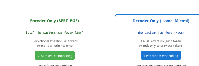
16.5.2 Encoder-Only vs. Decoder-Only for Embeddings
Historically, encoder-only models (BERT, RoBERTa) dominated the embedding space because their bidirectional architecture naturally produces rich token representations. Decoder-only models (GPT, Llama) are autoregressive and were not originally designed for embeddings. However, recent work has shown that decoder-only models can produce competitive embeddings with the right training approach. Figure 16.5.1a compares the two embedding extraction strategies.
| Aspect | Encoder-Only | Decoder-Only |
|---|---|---|
| Architecture | Bidirectional (BERT, RoBERTa) | Causal/autoregressive (Llama, Mistral) |
| Pooling strategy | [CLS] token or mean pooling | Last token or mean pooling |
| Typical model size | 100M to 400M parameters | 1B to 70B parameters |
| Embedding dimension | 768 to 1024 | 2048 to 8192 |
| Max sequence length | 512 tokens (typical) | 4K to 128K tokens |
| Inference speed | Fast (small model) | Slower (large model) |
| Quality for retrieval | Excellent with fine-tuning | Competitive with fine-tuning |
| Best for | High-throughput retrieval | When you already have the model deployed |
16.5.3 Contrastive Learning for Embeddings
The standard approach for fine-tuning embedding models is contrastive learning. The core idea is simple: train the model so that embeddings of semantically similar texts are close together, while embeddings of dissimilar texts are far apart. Training pairs can be constructed manually or generated using synthetic data techniques, and the model is optimized with a contrastive loss function. Code Fragment 16.5.3 shows this approach in practice.
The "why" behind contrastive over plain regression. You could imagine simply regressing pairs onto a target cosine similarity (1.0 for similar, 0.0 for dissimilar) with MSE loss; this used to be tried, and it underperforms. The reason is that retrieval cares about rank, not absolute similarity values: it does not matter whether the correct doc scores 0.83 or 0.91, only that it scores higher than every distractor. Contrastive losses optimize directly for this ranking property by comparing the positive to the negatives within the same softmax, so the gradient pushes the positive above the others rather than toward an arbitrary numeric target. The "ranking by construction" property is also why one well-chosen hard negative is worth dozens of random negatives: hard negatives are the ones the current model gets wrong, so the loss is non-zero and gradient signal is rich.
16.5.3.0 The Contrastive Objective: InfoNCE and Triplet Loss
To make "pull positives together, push negatives apart" precise enough to differentiate and minimize, we need the loss in closed form. The dominant choice is InfoNCE (also called NT-Xent, the normalized temperature-scaled cross-entropy loss). For a single anchor $a$ with a designated positive $p$ and a set of negatives $\{n\}$, it is the cross-entropy of a softmax over similarity scores:
Read the formula one piece at a time. The similarity is cosine, $\operatorname{sim}(u, v) = u^{\top} v / (\|u\|\,\|v\|)$, so it lives in $[-1, 1]$ and ignores vector magnitude. The numerator rewards a high anchor-positive similarity: minimizing the loss drives $\operatorname{sim}(a, p)$ up, which geometrically pulls the positive's embedding toward the anchor's. The denominator sums over the positive plus every negative, so it acts as a normalizer; the only way to shrink the loss without bound is to make the positive term dominate the sum, which means simultaneously pushing every $\operatorname{sim}(a, n)$ down. The temperature $\tau$ (typically $0.05$ to $0.1$) controls sharpness: dividing by a small $\tau$ amplifies score differences, so the softmax concentrates on the single closest candidate and the loss penalizes hard negatives heavily; a large $\tau$ flattens the distribution and treats all candidates more uniformly. InfoNCE is exactly the multi-class cross-entropy you would use to classify "which of these $1 + |\{n\}|$ candidates is the true positive," which is why the softmax framing makes it a ranking objective by construction.
An older alternative is the triplet loss, which drops the softmax and instead enforces a fixed margin $m$ between the anchor-positive distance and the anchor-negative distance:
where $d(\cdot, \cdot)$ is a distance (Euclidean or $1 - \operatorname{sim}$). The loss is zero once the positive is closer than the negative by at least the margin $m$, so it stops pushing on triplets the model already ranks correctly and focuses gradient on violated triplets. The practical drawback versus InfoNCE is that triplet loss compares the anchor to one negative at a time, so it needs explicit hard-negative mining to stay informative, whereas InfoNCE compares against a whole pool of negatives in a single step.
In-Batch Negatives and Why Batch Size Matters
Where does the negative pool $\{n\}$ come from in practice? The dominant trick is in-batch negatives: for a mini-batch of $B$ anchor-positive pairs, the positive of every other pair in the batch is reused as a negative for the current anchor. One forward pass over $B$ pairs therefore yields $B - 1$ negatives per anchor for free, with no extra encoding cost. This makes the effective number of negatives scale with the batch size, so a batch of 256 gives each anchor 255 contrasting examples while a batch of 16 gives only 15.
The key assumption is that other batch members are genuinely dissimilar to the current anchor. When that holds, larger batches sharpen the embedding space because the denominator in InfoNCE sums over more competitors and the loss stays meaningfully positive. This is the central failure mode of in-batch contrastive training: with a small batch the negative pool is tiny, the loss collapses toward zero, the gradient signal starves, and the model silently underperforms its own recipe. The opposite failure (a "false negative") occurs when two batch members actually are similar, since the loss then wrongly pushes them apart; deduplicating near-identical examples within a batch mitigates this. The dependence of quality on batch size is the reason production embedding training reaches for very large batches (sometimes via gradient accumulation or cross-device negative gathering) and why a contrastive run that worked in a paper can quietly degrade when someone shrinks the batch to fit a smaller GPU.
Code Fragment 16.5.2 below computes the symmetric NT-Xent loss for a small batch of normalized embeddings so the reader can watch the loss respond to the temperature and the number of in-batch negatives. (Section 31.1 covers the same InfoNCE objective from the vector-database angle, where it powers production embedding training at scale.)
# NT-Xent (InfoNCE) for a small batch of L2-normalized embeddings.
# anchors[i] and positives[i] form a positive pair; every other positive
# in the batch is an in-batch negative for anchor i. Pure PyTorch, no library loss.
import torch
import torch.nn.functional as F

torch.manual_seed(0)
batch_size, dim, tau = 4, 8, 0.07

# Two views of the same 4 items: positives[i] is the match for anchors[i].
anchors = F.normalize(torch.randn(batch_size, dim), dim=1)
noise = 0.1 * torch.randn(batch_size, dim)
positives = F.normalize(anchors + noise, dim=1)   # each positive sits near its anchor

# Cosine-similarity matrix (already unit vectors, so a dot product is the cosine).
logits = anchors @ positives.T / tau              # shape (B, B); diagonal = true pairs
labels = torch.arange(batch_size)                 # the positive for row i is column i

# Cross-entropy over each row IS InfoNCE: numerator = diagonal, denominator = whole row.
loss = F.cross_entropy(logits, labels)
print(f"in-batch negatives per anchor: {batch_size - 1}")
print(f"NT-Xent loss (tau={tau}): {loss.item():.4f}")
cross_entropy with diagonal labels is exactly the InfoNCE objective: the numerator is the true positive on the diagonal and the denominator is the whole row of in-batch candidates. Lowering tau or raising batch_size both increase the loss the model must work against, which is why temperature and batch size are the two knobs that most affect contrastive quality.16.5.3.1 Training Data: Pairs and Triplets
Code Fragment 16.5.2a loads the model via Section 3.1.
# Preparing contrastive training data
from dataclasses import dataclass
from typing import List, Optional
@dataclass
class ContrastivePair:
    """A pair of texts with a similarity label."""
    anchor: str # The query or reference text
    positive: str # Text that should be similar to anchor
    negative: str = None # Text that should be different (for triplet loss)
    score: float = 1.0 # Similarity score (0 to 1) for soft labels
    # Example: medical retrieval training data
    medical_pairs = [
        ContrastivePair(
        anchor="What are the symptoms of type 2 diabetes?",
        positive="Type 2 diabetes symptoms include increased thirst, frequent "
        "urination, blurred vision, fatigue, and slow wound healing.",
        negative="Type 1 diabetes is an autoimmune condition where the immune "
        "system attacks insulin-producing beta cells in the pancreas."
        ),
        ContrastivePair(
        anchor="Treatment options for hypertension",
        positive="First-line treatments for high blood pressure include ACE "
        "inhibitors, ARBs, calcium channel blockers, and thiazide "
        "diuretics, often combined with lifestyle modifications.",
        negative="Hypotension, or low blood pressure, is typically treated by "
        "increasing fluid intake and wearing compression stockings."
        ),
        ]
    # Convert to the format expected by Sentence Transformers
    def pairs_to_dataset(pairs: List[ContrastivePair]) -> dict:
        """Convert contrastive pairs to training format."""
        anchors = [p.anchor for p in pairs]
        positives = [p.positive for p in pairs]
        negatives = [p.negative for p in pairs if p.negative]
        if negatives:
            return {
                "anchor": anchors,
                "positive": positives,
                "negative": negatives,
                }
            return {
                "anchor": anchors,
                "positive": positives,
                }
# Fine-tune a sentence-transformer to your domain.
# CosineSimilarityLoss pulls similar-pair embeddings together and pushes
# dissimilar-pair embeddings apart.
from sentence_transformers import SentenceTransformer, losses, InputExample
from sentence_transformers.training_args import SentenceTransformerTrainingArguments
from sentence_transformers.trainer import SentenceTransformerTrainer
from torch.utils.data import DataLoader

model = SentenceTransformer("sentence-transformers/all-MiniLM-L6-v2")

# Each example: two sentences plus a similarity label in [0, 1]
train_examples = [
    InputExample(texts=["The cat sits on the mat.",
                        "A cat is on the rug."],            label=0.92),
    InputExample(texts=["The cat sits on the mat.",
                        "Stock prices fell sharply today."], label=0.05),
    InputExample(texts=["BERT uses masked language modeling.",
                        "BERT trains by predicting masked tokens."], label=0.95),
]

train_dataloader = DataLoader(train_examples, shuffle=True, batch_size=16)
train_loss = losses.CosineSimilarityLoss(model)

args = SentenceTransformerTrainingArguments(
    output_dir="./tuned-embedder",
    num_train_epochs=4,
    learning_rate=2e-5,
    per_device_train_batch_size=16,
    warmup_ratio=0.1,
)
trainer = SentenceTransformerTrainer(model=model, args=args,
                                     train_dataset=train_examples, loss=train_loss)
trainer.train()
model.save_pretrained("./tuned-embedder")sentence-transformers. The CosineSimilarityLoss trains the model to produce embeddings where similar pairs have high cosine similarity and dissimilar pairs have low similarity.The sentence-transformers library (pip install sentence-transformers) provides the most streamlined way to fine-tune embedding models with contrastive learning. It handles batching, loss computation, and in-batch negative mining automatically.
Show code
# pip install sentence-transformers
from sentence_transformers import SentenceTransformer, InputExample, losses
from torch.utils.data import DataLoader
model = SentenceTransformer("BAAI/bge-base-en-v1.5")
train_examples = [
    InputExample(texts=[pair.anchor, pair.positive, pair.negative])
    for pair in medical_pairs
]
loader = DataLoader(train_examples, batch_size=32, shuffle=True)
# MultipleNegativesRankingLoss uses in-batch negatives
loss = losses.MultipleNegativesRankingLoss(model)
model.fit(
    train_objectives=[(loader, loss)],
    epochs=2,
    warmup_steps=100,
    output_path="./medical-embeddings",
)
Code Fragment 16.5.3a provides a decision helper that weighs baseline performance gaps, corpus size, available training pairs, and reindexing costs to recommend whether embedding fine-tuning is worth the investment.
# Practical: deciding whether to fine-tune embeddings
def should_finetune_embeddings(
    baseline_ndcg: float,
    target_ndcg: float,
    corpus_size: int,
    num_training_pairs: int,
    reindex_cost_hours: float,
    ) -> dict:
    """Decision helper for embedding fine-tuning."""
    gap = target_ndcg - baseline_ndcg
    has_enough_data = num_training_pairs >= 1000
    gap_is_significant = gap > 0.05
    recommendation = "off-the-shelf"
    reasons = []
    if not gap_is_significant:
        reasons.append("Gap to target is small (<5%); fine-tuning unlikely to help")
    elif not has_enough_data:
        reasons.append("Need at least 1,000 training pairs; consider generating "
            "synthetic pairs with an LLM")
        recommendation = "generate_data_first"
    else:
        expected_improvement = min(gap * 1.5, 0.25) # Conservative estimate
        expected_ndcg = baseline_ndcg + expected_improvement
        if expected_ndcg >= target_ndcg:
            recommendation = "fine-tune"
            reasons.append(f"Expected NDCG after fine-tuning: ~{expected_ndcg:.2f}")
        else:
            recommendation = "fine-tune + improve retrieval pipeline"
            reasons.append("Fine-tuning alone may not close the gap; "
                "consider hybrid retrieval (BM25 + dense)")
            reasons.append(f"Reindexing will take ~{reindex_cost_hours:.1f} hours "
                f"for {corpus_size:,} documents")
            return {
                "recommendation": recommendation,
                "baseline": baseline_ndcg,
                "target": target_ndcg,
                "gap": gap,
                "reasons": reasons,
                }
            result = should_finetune_embeddings(
                baseline_ndcg=0.38,
                target_ndcg=0.55,
                corpus_size=500_000,
                num_training_pairs=5_000,
                reindex_cost_hours=3.5,
                )
            for k, v in result.items():
print(f" {k}: {v}")Save a checkpoint at least every epoch, and keep the best 3 by validation loss. Fine-tuning runs are short but the optimal stopping point is hard to predict. Having checkpoints lets you recover the best model without re-running.
16.5.4 Canonical Sentence-Embedding Recipes
The contrastive framing above is generic. In practice, four named recipes dominate the literature and most practitioners' tool belts. Each solves a different data-availability problem, and together they form the menu a team picks from when adapting embeddings to a new domain.
16.5.4.1 SBERT: Siamese Bi-Encoder Trained on NLI
Sentence-BERT (SBERT) (Reimers and Gurevych, 2019) is the original recipe and still the conceptual backbone of the entire sentence-transformers library. The architecture is a siamese bi-encoder: two BERT towers with tied weights (they are literally the same network, called twice), each producing a pooled sentence embedding via mean-over-tokens. The two embeddings are then compared with cosine similarity.
The training trick is to bootstrap sentence semantics from a labeled corpus that was not designed for embeddings at all: NLI (Natural Language Inference) datasets (SNLI and MultiNLI), which annotate sentence pairs as entailment, contradiction, or neutral. SBERT treats entailment pairs as positives, contradiction pairs as hard negatives, and trains with a classification head (predicting the NLI label from the two embeddings) or a triplet loss. Why this works is itself the punchline of the SBERT paper: NLI is a proxy task that forces the model to compress sentence meaning into a single vector before comparison, exactly what an embedding model must do at retrieval time. Figure 16.5.2c sketches the siamese architecture: two tied BERT towers process sentences A and B independently, mean-pool to vectors $u$ and $v$, and feed the concatenation $[u; v; |u-v|]$ to a 3-way softmax head during training.
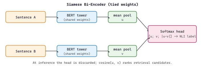
The SBERT paper's contribution was less the loss and more the architecture. Plain BERT is a cross-encoder: it scores a pair by passing both sentences through the network jointly (concatenated with [SEP]), so $N$ documents and $M$ queries require $N \times M$ forward passes. SBERT is a bi-encoder: each sentence is encoded once and the comparison is a cheap cosine, so $N + M$ forward passes suffice. The bi-encoder is what makes vector search practical at billion-document scale; the cross-encoder is still the gold standard for accuracy and is the right tool when you can afford to re-rank a small candidate list.
Training an SBERT model on NLI takes only a few lines with the sentence-transformers library. Code Fragment 16.5.4 shows the canonical NLI recipe with the siamese softmax loss.
# Canonical SBERT training on NLI pairs with the softmax loss.
from sentence_transformers import SentenceTransformer, InputExample, losses
from torch.utils.data import DataLoader
from datasets import load_dataset

base = SentenceTransformer("bert-base-uncased")  # two tied towers share these weights
nli = load_dataset("snli", split="train").filter(lambda r: r["label"] != -1)

# NLI labels: 0 = entailment (positive), 1 = neutral, 2 = contradiction (hard negative)
examples = [InputExample(texts=[r["premise"], r["hypothesis"]], label=r["label"]) for r in nli.select(range(20000))]
loader = DataLoader(examples, batch_size=64, shuffle=True)

# SoftmaxLoss concatenates [u; v; |u - v|] and trains a 3-way head on the NLI label.
loss = losses.SoftmaxLoss(base, sentence_embedding_dimension=base.get_sentence_embedding_dimension(), num_labels=3)
base.fit(train_objectives=[(loader, loss)], epochs=1, output_path="./sbert-nli")
base, so each pair triggers two forward passes that produce embeddings $u$ and $v$; the SoftmaxLoss head learns to classify entailment vs neutral vs contradiction from the concatenation $[u; v; |u - v|]$. After training, only the encoder is kept and downstream code calls base.encode(...).At deployment, using a published SBERT checkpoint takes three lines: load the model, encode a list of sentences, and score similarity with a cosine. Code Fragment 16.5.4b shows this inference pattern with the canonical lightweight checkpoint.
# Inference with a pretrained SBERT checkpoint: load, encode, compare.
from sentence_transformers import SentenceTransformer
from sentence_transformers.util import cos_sim

model = SentenceTransformer("sentence-transformers/all-MiniLM-L6-v2")
embeddings = model.encode(["cat", "dog", "automobile"])  # shape (3, 384)
similarity = cos_sim(embeddings[0], embeddings[1])        # cat vs dog
print(f"cos(cat, dog) = {similarity.item():.3f}")          # roughly 0.5
print(f"cos(cat, car) = {cos_sim(embeddings[0], embeddings[2]).item():.3f}")
Code Fragment 16.5.4b: SBERT at inference time. The all-MiniLM-L6-v2 checkpoint produces 384-dimensional sentence embeddings in a single batched encode call; downstream code stores those vectors in a vector index and ranks neighbours by cosine similarity.
16.5.4.2 Semi-Supervised Gold-to-Silver Bootstrapping
Most domain teams have at most a few thousand human-labeled similarity pairs and millions of unlabeled domain sentences. The gold-to-silver bootstrapping recipe turns the unlabeled mountain into training data using a high-quality but slow cross-encoder as the labeler.
- Train (or download) a gold cross-encoder. A cross-encoder fine-tuned on STSB or domain pairs gives accurate similarity scores but is too slow to deploy at retrieval time.
- Generate a balanced silver candidate pool. For each unlabeled sentence, retrieve $k$ nearest neighbours in an existing embedding space, then deliberately balance the sampling so the candidate pool covers the full similarity spectrum (very similar, mildly similar, dissimilar). Naive nearest-neighbour sampling alone over-represents the head and starves the contrastive loss of variety.
- Label the silver pool with the gold cross-encoder. The cross-encoder runs once, offline, producing scalar similarity scores for every candidate pair.
- Train the deployable bi-encoder on the silver dataset. Use any contrastive loss (CosineSimilarity, MultipleNegativesRanking, triplet). The fast SBERT-style student inherits the slow cross-encoder's domain knowledge without inheriting its inference cost.
This pattern is essentially knowledge distillation applied to retrieval. The balanced-NN sampling step is the underappreciated trick: it is the difference between a silver corpus that meaningfully teaches the student and one that simply confirms what the off-the-shelf embedder already knew.
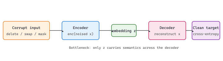
16.5.4.3 SDAE: Unsupervised Sentence Denoising
When no labels exist at all, the Sequential Denoising Autoencoder (SDAE) (Hill et al., 2016) provides a fully unsupervised signal. The recipe is a textbook autoencoder for sentences:
- Corrupt the input sentence by deleting, swapping, or masking a fraction of tokens.
- Pass the corrupted sentence through an encoder that produces a single sentence embedding.
- Train a decoder (often a small transformer) to reconstruct the original sentence from the embedding alone.
For the decoder to succeed, the embedding has to hold the full semantic content of the sentence. SDAE thus learns a representation that is sufficient for reconstruction, which tends to be a good general-purpose embedding even without any pair-similarity supervision. SDAE is most useful as a domain pretraining step on raw domain text, after which a small amount of labeled data unlocks contrastive fine-tuning.
The SDAE training objective is a standard reconstruction loss applied to the corrupted-input, clean-target pair $(\tilde{x}, x)$:
where $\tilde{x}$ is the noised sentence (token deletion, swap, or mask), $\operatorname{enc}_\phi(\tilde{x})$ is the pooled sentence embedding the model is forced to rely on, and the decoder generates the original tokens left-to-right. Gradient pressure on $\phi$ comes entirely from the bottleneck: the only way to reduce reconstruction loss is to pack enough semantics into the single embedding vector. Figure 16.5.3a shows the flow.
Code Fragment 16.5.4 sketches a minimal SDAE training step in PyTorch: token deletion supplies the corruption, an encoder pools the noised sentence to a single embedding, and a small transformer decoder is asked to regenerate the clean sequence from that embedding alone.
import torch, random
from transformers import AutoTokenizer, AutoModel, AutoModelForCausalLM

tok = AutoTokenizer.from_pretrained("bert-base-uncased")
encoder = AutoModel.from_pretrained("bert-base-uncased")
decoder = AutoModelForCausalLM.from_pretrained("gpt2")

def drop_tokens(ids, p=0.1):
    return [t for t in ids if random.random() > p]

def sdae_step(sentence, opt):
    clean = tok(sentence, return_tensors="pt").input_ids[0]
    noised = torch.tensor([drop_tokens(clean.tolist())])
    z = encoder(noised).last_hidden_state.mean(dim=1)        # bottleneck embedding
    out = decoder(input_ids=clean.unsqueeze(0),
                  encoder_hidden_states=z.unsqueeze(1),
                  labels=clean.unsqueeze(0))                 # reconstruct clean
    out.loss.backward(); opt.step(); opt.zero_grad()
    return out.loss.item()
Code Fragment 16.5.4c: SDAE training step. Token-deletion corruption, a pooled encoder embedding, and a decoder that must reconstruct the original sequence. The encoder is the artifact kept for downstream sentence-similarity tasks.
Take the clean sentence "the radiology report indicates a small lesion in the left frontal lobe" (12 words). Apply token-deletion noise with $p = 0.2$: a typical sample drops two or three tokens, yielding for example "the report indicates small lesion the left lobe" (8 words). The encoder pools this corrupted input to a single 768-dimensional embedding $z$. The decoder then receives only $z$ (no copy of the noised text) and must regenerate the full 12-word clean sentence token by token. To predict "radiology" at position 1, $z$ must encode that the topic is medical imaging; to recover "frontal" before "lobe", $z$ must encode anatomical location. After enough such training pairs on a domain corpus, the encoder produces embeddings that pack enough semantics to reconstruct the missing words, which is exactly the property needed for retrieval and clustering downstream.
16.5.4.4 SimCSE: Dropout as Data Augmentation
SimCSE (Gao et al., 2021) reduces unsupervised sentence-embedding training to one delightful trick: feed the same sentence twice through a transformer with dropout enabled, treat the two slightly different output embeddings as a positive pair, and use all other sentences in the batch as negatives. That is the entire algorithm.
Dropout, which randomly zeros out a small fraction of activations on each forward pass, supplies just enough noise to produce two views of the same sentence that share semantics but differ in fine-grained detail. The contrastive loss pulls those views together while pushing the in-batch negatives apart. SimCSE matched or beat the supervised SBERT models on STSB despite using zero labels, which is why it has become the default unsupervised baseline whenever a new sentence-embedding paper is proposed. The supervised variant of SimCSE plugs in NLI pairs and was state of the art for several years. Figure 16.5.3b makes the dropout-as-augmentation trick concrete: the same sentence enters the encoder twice with different dropout masks, producing two embeddings that the contrastive loss then treats as a positive pair.
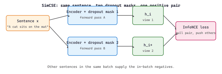
Formally, with a mini-batch of $N$ sentences and dropout-perturbed encodings $h_i$ and $h_i^{+}$ of the same sentence $x_i$, SimCSE minimises the symmetric InfoNCE loss:
$$\mathcal{L}_{\text{SimCSE}} = -\frac{1}{N}\sum_{i=1}^{N} \log \frac{\exp\!\big(\operatorname{sim}(h_i, h_i^{+}) / \tau\big)}{\sum_{j=1}^{N} \exp\!\big(\operatorname{sim}(h_i, h_j^{+}) / \tau\big)}$$
where $\operatorname{sim}(u, v) = u^{\top} v / (\|u\|\,\|v\|)$ is cosine similarity and the temperature $\tau$ (typically $0.05$) sharpens the softmax. The numerator pulls the two dropout views of $x_i$ together; the denominator pushes $h_i$ away from every other in-batch sentence's view. The whole training signal therefore lives inside the batch, which is why batch size acts as a quality knob.
Suppose a batch of $N = 4$ sentences produces cosine similarities (after dividing by $\tau = 0.05$) of $[16, 4, 5, 3]$ between anchor $h_1$ and the four candidates $h_1^{+}, h_2^{+}, h_3^{+}, h_4^{+}$. The softmax probability assigned to the true positive is $e^{16} / (e^{16} + e^{4} + e^{5} + e^{3}) \approx 0.99998$, giving a per-anchor loss of $-\log(0.99998) \approx 2\times 10^{-5}$. Shrink the batch to $N = 2$ and the same anchor sees only $[16, 4]$, dropping the loss further toward zero and starving the gradient. Bumping the batch to $N = 64$ adds 60 more competing negatives, which keeps the loss meaningfully positive and forces the encoder to sharpen its representations. This is why the original paper used batch size 64 to 512 and why a small-batch SimCSE run silently underperforms its own paper.
# SimCSE: the simplest unsupervised sentence embedding recipe in existence.
# Two forward passes of the same sentence under dropout give a positive pair.
from sentence_transformers import SentenceTransformer, losses, InputExample
from torch.utils.data import DataLoader

model = SentenceTransformer("bert-base-uncased")  # dropout=0.1 stays enabled at train time

# Each example is the *same sentence twice*: the dropout masks differ, the text doesn't.
train_examples = [
    InputExample(texts=[sent, sent]) for sent in unlabeled_domain_sentences
]
loader = DataLoader(train_examples, batch_size=64, shuffle=True)

# MultipleNegativesRankingLoss treats other in-batch sentences as negatives.
loss = losses.MultipleNegativesRankingLoss(model)
model.fit(train_objectives=[(loader, loss)], epochs=1, output_path="./simcse-domain")
Reusing a published SimCSE checkpoint is just as terse: load the supervised variant from the Hugging Face Hub and call encode. Code Fragment 16.5.5b shows the inference path.
# Loading a public SimCSE checkpoint and embedding a few sentences.
from sentence_transformers import SentenceTransformer
from sentence_transformers.util import cos_sim

model = SentenceTransformer("princeton-nlp/sup-simcse-bert-base-uncased")
sentences = ["A man is playing a guitar.", "Someone is strumming an instrument.", "A child rides a bike."]
vecs = model.encode(sentences)                       # shape (3, 768)
print(cos_sim(vecs[0], vecs[1]).item())              # high: paraphrase
print(cos_sim(vecs[0], vecs[2]).item())              # low: unrelated
Code Fragment 16.5.5b: Inference with the supervised SimCSE checkpoint. The 768-dimensional embeddings rank paraphrases above unrelated sentences with no further training.
16.5.4.5 Which Recipe When?
| Recipe | Labels Needed | Best For | Watch Out For |
|---|---|---|---|
| SBERT (NLI) | NLI-style entailment / contradiction | General-purpose English embeddings | Domain shift if your text is far from NLI |
| Gold-to-Silver Bootstrap | Small gold set + lots of unlabeled domain text | Domain adaptation with limited labels | Cross-encoder labeling cost; balance the silver pool |
| SDAE | None | Pure-text domains (legal, medical) with no labels at all | Decoder training cost; weaker than contrastive at the end |
| SimCSE (unsupervised) | None | Quick unsupervised baseline; works surprisingly well | Tune batch size; small batches starve the in-batch negatives |
| SimCSE (supervised) | NLI pairs | State-of-the-art with NLI labels | Same NLI domain caveat as SBERT |
16.5.5 Evaluating Embeddings: STSB and MTEB
Two benchmarks dominate sentence-embedding evaluation, and both should appear in every embedding fine-tuning project's report.
16.5.5.1 STSB: Semantic Textual Similarity Benchmark
STSB pairs English sentences with a human-assigned similarity score from 1 (unrelated) to 5 (semantically equivalent). The score is a Mean Opinion Score (MOS): each pair was rated by five annotators and the score is their average. The headline metric is Spearman rank correlation between the model's cosine similarities and the human MOS scores. Spearman, not Pearson, is the right choice: retrieval cares about ranking, and Spearman measures rank agreement directly. A Spearman of 0.85 is roughly the ceiling humans agree with each other, so models reporting 0.86 on STSB are essentially at the inter-annotator-agreement noise floor.
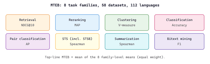
16.5.5.2 MTEB: Massive Text Embedding Benchmark
MTEB (Muennighoff et al., 2023) is the embedding equivalent of GLUE: a single leaderboard that aggregates 58 datasets across 8 task families (retrieval, reranking, clustering, classification, pair classification, semantic textual similarity, summarization, bitext mining) covering 112 languages. The MTEB score is the average across the 8 task families, computed per-language for multilingual models. Crucially, STSB lives inside MTEB as one of many tasks, which means the MTEB top-line score implicitly includes STSB performance and a great deal more. The aggregation rule is a two-level mean: first average within each task family $T_f$, then average across the eight families:
$$\text{MTEB} = \frac{1}{8}\sum_{f=1}^{8}\frac{1}{|T_f|}\sum_{d \in T_f} s_d$$
where $s_d$ is the per-dataset primary metric (NDCG@10 for retrieval, V-measure for clustering, accuracy for classification, Spearman for STS, and so on). The outer 1/8 weighting equalizes the eight families regardless of how many datasets each contains, which prevents the retrieval-heavy task families from drowning out clustering or bitext mining. Figure 16.5.4d shows the eight families that feed into the top-line score.
For practitioners, the practical advice is simple: report MTEB if the team is releasing a general-purpose embedding model, report a domain-specific Recall@k or NDCG@k on a held-out test set if the team is fine-tuning for a single application, and use STSB Spearman as the quickest possible sanity check that a fresh fine-tune did not silently collapse the embedding space. The MTEB leaderboard at HuggingFace is also the right place to pick a starting checkpoint: BGE, GTE, and E5 families all publish their MTEB scores so a team can choose the strongest base for their planned fine-tune. Code Fragment 16.5.5c shows the minimal MTEB invocation: pick one task, hand it a sentence-transformer, and call run.
# Smallest possible MTEB run: one task, one model, one score.
from mteb import MTEB
from sentence_transformers import SentenceTransformer

model = SentenceTransformer("sentence-transformers/all-MiniLM-L6-v2")
benchmark = MTEB(tasks=["Banking77Classification"])
results = benchmark.run(model, output_folder="./mteb-banking77")
print(results)
Code Fragment 16.5.5c: Minimal MTEB invocation against a single classification task. Subsetting to one task gives a fast smoke test before launching the full 58-dataset benchmark.
Show code
# pip install mteb
from mteb import MTEB
from sentence_transformers import SentenceTransformer

model = SentenceTransformer("./medical-embeddings")  # your fine-tuned model
evaluation = MTEB(tasks=["STSBenchmark", "TwentyNewsgroupsClustering", "AmazonPolarityClassification"])
results = evaluation.run(model, output_folder="./mteb-results")
print({task: round(r["test"]["main_score"], 3) for task, r in results.items()})
SentenceTransformer-compatible model across the full benchmark. Subset to the tasks closest to your application to get a fast, domain-relevant signal.Who: A search engineering team at an intellectual property analytics firm building a prior art search engine over 8 million patent documents.
Situation: Their search system used off-the-shelf BGE-large embeddings for semantic search. Patent examiners reported that the system missed relevant prior art in 35% of test queries because general-purpose embeddings did not capture patent-specific similarity (e.g., that "fastening mechanism" and "bolt assembly" describe related inventions).
Problem: Patent language is highly specialized, with domain-specific synonyms, technical jargon, and a unique notion of "similarity" based on functional equivalence rather than lexical overlap. Off-the-shelf embeddings were trained on web text and did not capture these relationships.
Dilemma: They could use BM25 keyword search as a fallback (misses semantic matches), expand queries with an LLM (adds latency, expensive at scale), or fine-tune the embedding model on patent-specific similarity pairs.
Decision: They fine-tuned BGE-large using contrastive learning on 25,000 patent similarity pairs generated from patent citation networks (if patent A cites patent B, they are a positive pair) and examiner relevance judgments from their historical search logs.
How: They used MultipleNegativesRankingLoss with in-batch negatives, training for 5 epochs on a single A100 GPU (8 hours). Hard negatives were patents from the same IPC class that were not cited by the query patent. After training, they reindexed all 8 million patents (a 36-hour batch job).
Result: Recall@20 improved from 65% to 84% on a test set of 1,000 examiner-validated queries. The fine-tuned model correctly captured patent-specific similarity: "fastening mechanism" now retrieved "bolt assembly," "adhesive bonding system," and "clip attachment device." The reindexing cost was $800 in compute, and ongoing inference cost was identical to the original model.
Lesson: Fine-tuned embeddings are essential when your domain has a specialized notion of similarity that differs from general text; citation networks and historical relevance judgments are excellent sources of training signal for domain-specific embedding models.
Fine-tuning embeddings for a specific domain is like recalibrating a telescope for a particular region of the sky. The general-purpose instrument works fine for stargazing, but the specialized one reveals details that were previously invisible. The catch? Every time you recalibrate, you need to re-photograph the entire sky (reindex your corpus).
Contrastive fine-tuning methods like GISTEmbed and instructor-based approaches are producing task-aware embeddings that outperform general-purpose embedding models on domain-specific retrieval. Research on matryoshka representation learning creates embeddings where subsets of dimensions form valid lower-dimensional representations, enabling flexible accuracy-latency tradeoffs at inference time.
The frontier is learning representations that capture both semantic similarity and structured relational knowledge (such as hierarchical or causal relationships) in a single embedding space.
- Fine-tuned embeddings provide 30% to 70% improvement over off-the-shelf models in specialized domains where vocabulary and similarity notions differ from general text.
- Encoder-only models (BERT, BGE) remain the practical choice for high-throughput embedding tasks due to their small size and fast inference; decoder-only models are competitive but slower.
- Contrastive learning with MultipleNegativesRankingLoss is the standard approach: it uses in-batch negatives to create a strong training signal without explicit hard negative mining.
- You need at least 1,000 training pairs for effective fine-tuning; if you have fewer, generate synthetic pairs using an LLM before fine-tuning.
- Always benchmark off-the-shelf first to measure the actual performance gap before investing in fine-tuning and the associated reindexing costs.
- Reindexing is a hidden cost: switching to a fine-tuned embedding model requires recomputing embeddings for your entire corpus, which must be planned into the deployment timeline.
Show Answer
Show Answer
Show Answer
Show Answer
Show Answer
Exercises
Explain the difference between fine-tuning for generation (SFT) and fine-tuning for representation learning. What is the output of a representation model?
Answer Sketch
SFT trains the model to generate text sequences; the output is generated tokens. Representation fine-tuning trains the model to produce meaningful embedding vectors; the output is a fixed-size dense vector for each input. The embedding should place semantically similar inputs near each other in vector space. Representation models are used for search, retrieval, clustering, and as features for downstream classifiers.
Describe how contrastive learning works for training embedding models. What are positive and negative pairs, and why is the choice of negatives important?
Answer Sketch
Contrastive learning pulls positive pairs (semantically similar) together and pushes negative pairs (dissimilar) apart in embedding space. Positive pairs: a question and its relevant document. Negatives: a question paired with an irrelevant document. Hard negatives (documents that are similar but not relevant) are crucial because they force the model to learn fine-grained distinctions. Easy negatives (completely unrelated documents) provide little learning signal since the model already separates them.
Explain the Matryoshka Representation Learning (MRL) technique. Write pseudocode for a training loop that produces embeddings usable at multiple dimensionalities (64, 128, 256, 768).
Answer Sketch
MRL trains the model so that the first N dimensions of the embedding are useful on their own, for any N. Training: for each batch, compute the full embedding, then apply the contrastive loss at multiple truncation points: for dim in [64, 128, 256, 768]: loss += contrastive_loss(embeddings[:, :dim], labels). At inference, truncate to the desired dimensionality based on storage/speed requirements. Lower dims trade quality for 4 to 12x space savings.
A legal search engine uses a general-purpose embedding model but struggles with queries about specific contract clauses. How would you fine-tune the embedding model for this domain? What training data would you need?
Answer Sketch
Collect training pairs: (query, relevant contract clause) as positives. Generate hard negatives: clauses that mention similar terms but answer different questions. Fine-tune with contrastive loss for 1 to 3 epochs with a low learning rate (1e-5). Evaluate on a held-out set of legal queries with known relevant clauses using recall@k and NDCG. The key is hard negatives from the legal domain, which teach the model to distinguish between similar but legally distinct concepts.
Write a function that evaluates embedding quality on an information retrieval task. Compute recall@1, recall@5, recall@10, and Mean Reciprocal Rank (MRR) given queries, document embeddings, and relevance labels.
Answer Sketch
For each query: compute cosine similarity with all documents, rank by similarity. recall_at_k = 1 if any relevant doc in top-k else 0. reciprocal_rank = 1/rank_of_first_relevant_doc. Average across all queries for each metric. Use numpy: sims = query_emb @ doc_embs.T; ranked = np.argsort(-sims). Report all four metrics; MRR is the most informative single metric for ranking quality.
What Comes Next
In the next section, Section 16.6: Fine-Tuning for Classification & Sequence Tasks, we cover fine-tuning for classification and sequence labeling tasks. The contrastive training data preparation connects to embedding training methods in Section 31.3 and the data curation pipelines in Section 6.4, the most common supervised NLP applications.
For the embedding-and-retrieval stack that fine-tuned representations plug into, see Section 31.1: Embeddings and Vector Databases. For the InfoNCE and hard-negative-mining recipes that every modern embedder is trained with, see Section 36.4: Models. For the MTEB-and-BEIR benchmarks you measure a fine-tuned embedder against, see Section 36.3: Datasets and Benchmarks.