Your language model is secretly a reward model. You just need the right loss function to reveal it.
Reward, Secretly Rewarding AI Agent
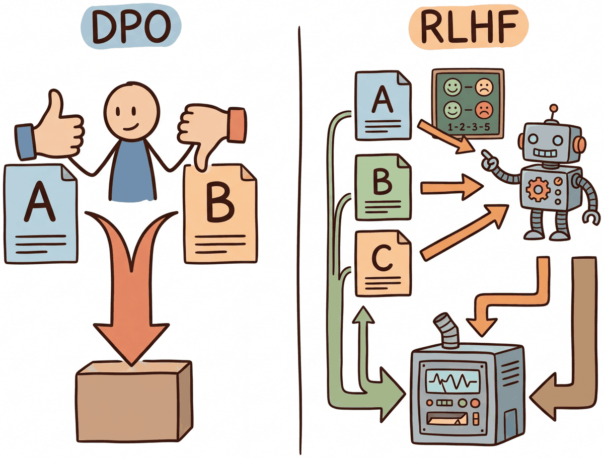
DPO achieves RLHF-level alignment without reinforcement learning. The key insight is mathematical: the optimal policy under the RLHF objective has a closed-form relationship with the reward function. This can be implemented efficiently using parameter-efficient methods like LoRA. This means you can reparameterize the reward model loss directly in terms of the policy, training the language model on preference pairs using a simple classification-like objective. No reward model, no RLHF, no value network. Building on the RLHF pipeline from Section 18.1, this dramatically simplifies the alignment pipeline and has spawned an entire family of "direct alignment" methods (KTO, ORPO, SimPO, IPO) that each address different limitations of the original formulation.
Prerequisites
This section continues from Section 18.3. You should be comfortable with RLHF from Section 18.1 and with supervised fine-tuning from Section 16.1. The DPO loss derivation builds on the cross-entropy and probability-ratio intuitions from Chapter 0.
This continuation of Section 18.3 picks up after the DPO derivation and explores the family of methods that have followed. It covers the DPO variants (KTO, IPO, ORPO, SimPO) that each address a specific limitation of the original formulation, how preference datasets are created and synthesized in practice, the practical training considerations that decide whether a DPO run actually works, and the online and iterative variants that push past a single offline training pass.
18.4.1 DPO Variants and Extensions
DPO (Direct Preference Optimization, Rafailov et al., 2023) was framed in the original paper as a "closed-form solution to RLHF", and the closed-form derivation famously fits on a single slide. The paper was rejected from one major conference in early 2023 before being accepted at NeurIPS 2023, where it won the Outstanding Main Track Paper award. GRPO arrived shortly after via DeepSeek-R1 and now competes with DPO as the default fine-tuning loss in most open-source training stacks.
Log the mean chosen reward minus rejected reward at each step. This margin should grow during healthy DPO training. A margin stuck near zero means the model is not differentiating between chosen and rejected responses, even if the loss is decreasing (the loss can decrease by reducing confidence in BOTH responses equally). TRL's DPOTrainer logs this as rewards/margins; make it a primary dashboard metric, not just a sanity check.
The success of DPO inspired a wave of variants, each addressing specific limitations. It is worth noting that DPO does not universally match RLHF quality: on complex tasks requiring long outputs or nuanced reasoning, PPO-based RLHF can still outperform DPO, likely because the separate reward model provides a richer optimization signal. The core differences among DPO variants lie in data requirements, loss formulations, and training dynamics.
For verifiable-reward tasks (math, code, JSON output), trl's GRPOTrainer replaces the value head with group-relative advantages, cutting RLHF memory by ~25% vs PPO. Define a Python reward_funcs callable that scores generations, pass it to GRPOConfig, and the trainer samples num_generations rollouts per prompt and normalizes inside the group. This is the recipe behind DeepSeek-R1 reasoning fine-tunes.
Show code
pip install trl
from trl import GRPOTrainer, GRPOConfig
def reward_len(completions, **kwargs):
    return [-abs(20 - len(c)) for c in completions]
cfg = GRPOConfig(output_dir="grpo-out", num_generations=8,
                 learning_rate=1e-6, per_device_train_batch_size=4)
trainer = GRPOTrainer(model=model, reward_funcs=reward_len,
                      args=cfg, train_dataset=ds)
trainer.train()18.4.1.1 KTO: Kahneman-Tversky Optimization
KTO (Ethayarajh et al., 2024) addresses a practical limitation of DPO: the requirement for paired preferences. In real applications, feedback often comes as binary signals (thumbs up or thumbs down) rather than pairwise comparisons. KTO works with unpaired binary feedback, using ideas from prospect theory to weight losses and gains asymmetrically. Code Fragment 18.4.5 demonstrates KTO training with TRL.
The implicit reward of a response $y$ under the policy $\pi_\theta$ and reference $\pi_{\mathrm{ref}}$ is
and the KTO loss treats desirable and undesirable examples asymmetrically using a Kahneman-Tversky value function $v$:
where $\ell \in \{\text{desirable}, \text{undesirable}\}$, $\lambda_\ell$ is the per-label weight (the desirable_weight / undesirable_weight hyperparameters), and $z_0 = \beta \,\mathrm{KL}\!\big(\pi_\theta \| \pi_{\mathrm{ref}}\big)$ is a reference KL anchor. The value function $v(z) = \sigma(z)$ for desirable examples and $v(z) = \sigma(-z)$ for undesirable ones, encoding loss-aversion in the same way as prospect theory.
An AI assistant team logs 100 K user interactions: 28 K thumbs-up, 14 K thumbs-down, 58 K with no rating. To run DPO they would need to discard everything that is not paired with both a chosen and a rejected response, leaving only the prompts that received both signals (roughly 4 K pairs). KTO instead uses all 42 K labelled examples directly, with $\lambda_{\mathrm{des}} = 1.0$ and $\lambda_{\mathrm{undes}} = 14/28 = 0.5$ so the loss does not over-weight the rarer negative class. On HH-RLHF style benchmarks this 10x increase in usable data yields a 4 to 8 point gain in win rate over a DPO baseline trained on the paired subset (Ethayarajh et al., 2024, Table 3).
from datasets import load_dataset
# KTO Training with TRL
from trl import KTOTrainer, KTOConfig
# KTO uses unpaired binary data
# Each example has: prompt, completion, label (True/False)
kto_dataset = load_dataset("trl-lib/kto-mix-14k", split="train")
print(f"Example: {kto_dataset[0]}")
# {'prompt': '...', 'completion': '...', 'label': True}
kto_config = KTOConfig(
output_dir="./kto-llama-8b",
beta=0.1,
desirable_weight=1.0, # weight for positive examples
undesirable_weight=1.0, # weight for negative examples
per_device_train_batch_size=4,
gradient_accumulation_steps=8,
learning_rate=5e-7,
num_train_epochs=1,
max_length=2048,
bf16=True,
)
kto_trainer = KTOTrainer(
model=model,
ref_model=ref_model,
args=kto_config,
train_dataset=kto_dataset,
tokenizer=tokenizer,
)
kto_trainer.train()
Example: {'prompt': 'Write a short poem about spring.', 'completion': 'Blossoms unfurl...', 'label': True}
{'train_loss': 0.4917, 'train_runtime': 487.3}
18.4.1.2 ORPO: Odds Ratio Preference Optimization
ORPO (Hong et al., 2024) eliminates the need for a separate reference model entirely. It combines the SFT objective with a preference optimization term in a single loss function. The key idea is to use the odds ratio of generating the chosen versus rejected response, contrasting them directly without a reference model baseline.
Define the odds of a response under the policy as $\mathrm{odds}_\theta(y \mid x) = \pi_\theta(y \mid x) \,/\, \big(1 - \pi_\theta(y \mid x)\big)$. ORPO trains on $(x, y_w, y_l)$ triples (chosen $y_w$, rejected $y_l$) with the joint loss
where $\lambda$ (typically $0.1$ to $1.0$) controls how strongly the model is penalised for assigning high odds to the rejected response. Because both terms depend only on $\pi_\theta$, no frozen reference copy is required.
ORPO's main advantage is memory efficiency. By removing the reference model, ORPO requires only a single model in GPU memory during training, making it practical for alignment of very large models on limited hardware. The tradeoff is that without a reference anchor, the optimization can be less stable than DPO for some tasks.
Fine-tuning a 7B model with DPO needs the trainable policy plus a frozen reference, roughly $7 \text{B} \times 2 \times 2 \text{B} = 28 \text{ GB}$ in BF16 even before optimiser states. ORPO halves this to about 14 GB, fitting comfortably on a single RTX 4090. A typical recipe is $\lambda = 0.5$, learning rate $5 \times 10^{-6}$, 1 epoch on UltraFeedback, and batches of 4 with gradient accumulation 8. Hong et al. (2024) report that Mistral-7B trained with ORPO matches Zephyr-beta (which used SFT then DPO) on MT-Bench while halving the training compute.
18.4.1.3 SimPO: Simple Preference Optimization
SimPO (Meng et al., 2024) also removes the reference model but takes a different approach. Instead of using log-probability ratios, SimPO uses the average log-probability of the response (normalized by length) as the implicit reward. It adds a target margin γ to the objective, encouraging a minimum quality gap between preferred and rejected responses.
Concretely, SimPO defines the implicit reward of a response of length $|y|$ as the length-normalised log-likelihood
and trains with a margin-augmented Bradley-Terry loss
where the target margin $\gamma > 0$ (typically $0.5$ to $1.5$) forces the chosen response to beat the rejected one by at least $\gamma$ nats before the loss saturates.
Suppose for prompt $x$ the policy assigns $\log \pi_\theta(y_w \mid x) = -45$ over $|y_w| = 90$ tokens and $\log \pi_\theta(y_l \mid x) = -36$ over $|y_l| = 60$ tokens. With $\beta = 2.0$, $r_\theta(x, y_w) = 2.0 \times (-45/90) = -1.0$ and $r_\theta(x, y_l) = 2.0 \times (-36/60) = -1.2$. The implicit margin is $-1.0 - (-1.2) = 0.2$. With target margin $\gamma = 0.5$ the loss is $-\log \sigma(0.2 - 0.5) = -\log \sigma(-0.3) \approx 0.85$, still pushing the policy to widen the gap even though the chosen response already has higher length-normalised likelihood. Plain DPO with the same scores would see the un-normalised gap of $-45 - (-36) = -9$ and incorrectly conclude that $y_l$ is preferred.
18.4.1.4 IPO: Identity Preference Optimization
IPO (Azar et al., 2024) addresses a theoretical issue with DPO: under certain conditions, DPO can overfit to preference data, driving the log-probability ratio to infinity. IPO uses a squared loss instead of the sigmoid loss, providing better regularization properties and more stable training.
Concretely, let $\rho_{\theta}(x, y) \,=\, \log\!\frac{\pi_{\theta}(y \mid x)}{\pi_{\text{ref}}(y \mid x)}$ be the implicit reward at a (prompt, response) pair. DPO uses a logistic loss on the preference margin $\rho_{\theta}(x, y_w) - \rho_{\theta}(x, y_l)$, which is unbounded above and rewards driving the margin to infinity once a pair is correctly ranked. IPO replaces it with a squared anchor loss
$$\mathcal{L}_{\text{IPO}}(\theta) \;=\; \mathbb{E}_{(x, y_w, y_l) \sim \mathcal{D}}\left[\Bigl(\rho_{\theta}(x, y_w) - \rho_{\theta}(x, y_l) - \tfrac{1}{2\beta}\Bigr)^{2}\right],$$
where the target margin $1/(2\beta)$ is determined by the KL-regularisation strength $\beta$ (the same $\beta$ as in DPO). The squared loss is bounded below by zero and bounded above by the square of the largest log-ratio in the batch, so no single example can dominate the gradient by being trivially separable. Once the margin reaches the anchor value, gradient flow stops; this is the formal sense in which IPO "regularises" the optimisation problem that DPO leaves underdetermined.
Suppose you have 800 preference pairs and a 7B base model. After 3 epochs of DPO with $\beta = 0.1$, you observe: train accuracy 100%, validation accuracy 71%, and the average implicit reward margin has ballooned to about $+18$ nats on the train set. The model now confidently outputs the chosen completion verbatim for almost any in-distribution prompt and degrades on held-out instructions; this is the textbook DPO over-fit failure mode. Re-running with IPO at the same $\beta$ produces train accuracy 93%, validation accuracy 78%, and a stable margin near $1/(2\beta) = 5$ nats throughout training. The reason is that IPO's squared loss has zero gradient at the anchor margin, so once the model has learned a separation of 5 nats it stops pushing further; DPO's sigmoid loss keeps a residual gradient that nudges the model toward infinite margins until the train accuracy hits 100%. Rule of thumb: prefer IPO when your preference dataset is smaller than $\sim 2{,}000$ pairs, when many pairs are trivial to separate, or when you observe the DPO training loss falling below 0.05.
| Method | Reference Model | Data Format | Key Advantage | Key Limitation |
|---|---|---|---|---|
| DPO | Required (frozen) | Pairwise (chosen/rejected) | Well-studied, strong baselines | Needs paired data + reference model |
| KTO | Required (frozen) | Binary (good/bad) | Works with unpaired feedback | Less data-efficient than pairwise |
| ORPO | Not needed | Pairwise (chosen/rejected) | Single model, combined SFT+alignment | Can be less stable |
| SimPO | Not needed | Pairwise (chosen/rejected) | Length-normalized, margin-based | Newer, less extensively validated |
| IPO | Required (frozen) | Pairwise (chosen/rejected) | Prevents overfitting, squared loss | May underfit with limited data |
18.4.2 Creating Preference Datasets
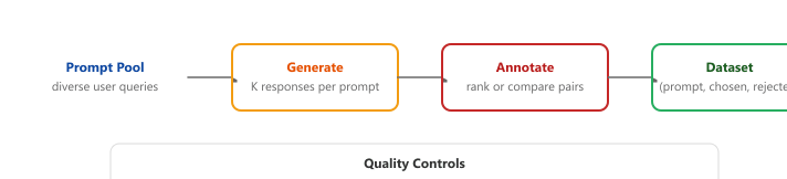
The quality of alignment training depends critically on the preference dataset. Creating high-quality preference data (using techniques from Section 15.2 on synthetic data pipelines) involves careful annotation design, quality control, and understanding of common pitfalls. Figure 18.4.2 outlines the preference data creation pipeline.
- Clear guidelines: Define specific criteria for what makes a response "better" (accuracy, helpfulness, safety, conciseness)
- Multiple annotators: Use at least 2-3 annotators per comparison to measure agreement
- Calibration: Include known-answer items to detect annotator drift
- Diversity: Ensure prompts span different tasks, difficulty levels, and domains
- Margin filtering: Remove pairs where responses are nearly identical in quality (low signal-to-noise)
Every preference dataset above asks the annotator to pick which of two responses is better, not to score either of them on an absolute 1-to-5 helpfulness scale. The reason is psychometric, not technical. Humans are demonstrably bad at producing well-calibrated absolute ratings: one annotator's "4" is another's "5", the same annotator's "4" drifts over the course of a labeling session, and the scale itself is anchored by whatever recent items the annotator just saw. Inter-annotator agreement on absolute 1-5 helpfulness ratings is typically Cohen's $\kappa \approx 0.3$ to $0.5$ (fair to moderate). The same annotators agree on pairwise "which is better" judgments at $\kappa \approx 0.7$ to $0.8$ (substantial). The classic psychophysics result is that humans excel at relative comparisons (A is taller than B, A is brighter than B) and struggle with absolute magnitude estimates, and the same pattern shows up in response quality judgments. The Bradley-Terry reward-model loss in Section 18.1.2.2 is what lets us recover absolute scalar rewards from pairwise judgments without ever asking annotators for absolute scores in the first place. This is also the reason RLHF, DPO, KTO, and ORPO all consume preference data, not scored data.
18.4.2.1 Stacking Multiple Reward Models
A single scalar reward model has to compress every alignment criterion (helpfulness, harmlessness, conciseness, format adherence, factual accuracy) into one number. In practice the criteria conflict: the most helpful response is often the longest, the most harmless one is often the most evasive, and the most concise one is often the least informative. A widely-used pattern is to train separate reward models per axis on preference data labeled for that axis alone, then combine them at PPO time into a composite reward:
Each $r_i$ is its own reward model (helpfulness, harmlessness, conciseness, etc.) and the weights $w_i$ are set by the model owner to encode the policy stance, for example $w_{\text{harmless}} = 2$ and $w_{\text{helpful}} = 1$ if safety should dominate. Anthropic's HH (Helpful + Harmless) work and Meta's Llama-2-Chat both ship two-headed reward models trained on disjoint preference datasets; the LLM-as-judge community routinely combines a "quality" RM with a "safety" RM at inference. The advantage over a single multi-objective RM is that each dataset can be smaller and easier to label, the weights $w_i$ can be retuned without re-training any RM, and the RM ensemble is far more robust to reward hacking (see Section 18.2): an adversarial response that fools the helpfulness RM rarely also fools the harmlessness RM at the same time. The trade-off is wall-clock cost: PPO now has to forward two or three frozen RMs per rollout instead of one.
18.4.3 Synthetic Preference Generation
Human annotation is expensive and slow. A growing trend is to generate synthetic preference data using a stronger model (such as GPT-4 or Claude) as the judge. This approach, sometimes called "AI feedback" or RLAIF (Section 18.5), can produce large preference datasets at a fraction of the cost of human annotation. Code Fragment 18.4.4 demonstrates this LLM-as-judge approach for building synthetic preference datasets.
import json
# Synthetic preference generation with LLM-as-judge
import openai
from dataclasses import dataclass
from typing import List, Tuple
@dataclass
class PreferencePair:
    prompt: str
    chosen: str
    rejected: str
    judge_rationale: str
    def generate_preference_pair(
        prompt: str,
        response_a: str,
        response_b: str,
        judge_model: str = "gpt-4o",
        ) -> PreferencePair:
        """Use a strong model to judge which response is better."""
        judge_prompt = f"""Compare these two responses to the given prompt.
        Evaluate on: accuracy, helpfulness, clarity, and safety.
        Return JSON with "winner" (A or B) and "rationale".
        Prompt: {prompt}
        Response A: {response_a}
        Response B: {response_b}"""
        client = openai.OpenAI()
        result = client.chat.completions.create(
            model=judge_model,
            messages=[{"role": "user", "content": judge_prompt}],
            response_format={"type": "json_object"},
            temperature=0.0,
            )
        judgment = json.loads(result.choices[0].message.content)
        if judgment["winner"] == "A":
            return PreferencePair(prompt, response_a, response_b, judgment["rationale"])
        else:
            return PreferencePair(prompt, response_b, response_a, judgment["rationale"])
        def build_synthetic_dataset(
            prompts: List[str],
            model_name: str = "meta-llama/Llama-3.1-8B-Instruct",
            samples_per_prompt: int = 4,
            ) -> List[PreferencePair]:
            """Build a preference dataset using rejection sampling + LLM judge."""
            import itertools
            pairs = []
            for prompt in prompts:
                # Generate multiple responses with different temperatures
                responses = []
                for temp in [0.3, 0.5, 0.7, 1.0]:
                    response = generate_response(model_name, prompt, temperature=temp)
                    responses.append(response)
                    # Create all pairwise comparisons
                    for a, b in itertools.combinations(responses, 2):
                        pair = generate_preference_pair(prompt, a, b)
                        pairs.append(pair)
                        return pairs
Dataset size: 500
Columns: ['source', 'chosen', 'rejected', 'prompt', 'chosen_rating', 'rejected_rating']

Prompt: Write a C++ function to find the longest common subsequence of two input strings...

Chosen: Here is a C++ function that finds the longest common subsequence using dynamic prog...

Rejected: You can find the longest common subsequence by comparing each character one by one...
Synthetic preferences inherit the biases of the judge model. If the judge systematically prefers verbose responses, the trained model will learn to be verbose. Always validate synthetic data against a held-out set of human preferences, and consider using multiple judge models to reduce individual model bias.
18.4.4 Practical Considerations for DPO Training
DPO is mathematically elegant, but practitioners discover quickly that it is also unusually sensitive to a small set of hyperparameters. The β coefficient, the learning rate, and the choice of reference model can each flip a training run from "matches PPO" to "model collapses to verbose nonsense." We focus on the three most impactful dials, beginning with β and its non-intuitive interaction with the implicit KL term.
18.4.4.1 Hyperparameter Sensitivity
DPO training is sensitive to several key hyperparameters. The most important is β, which controls the strength of the implicit KL constraint. A β that is too low leads to aggressive optimization that can degrade coherence. A β that is too high produces minimal change from the SFT model. Code Fragment 18.4.8 provides recommended hyperparameter ranges for DPO training.
# Hyperparameter sweep for DPO
from dataclasses import dataclass
from typing import List, Dict
@dataclass
class DPOSweepConfig:
    """Configuration for DPO hyperparameter search."""
    beta_values: List[float] = None
    learning_rates: List[float] = None
    warmup_ratios: List[float] = None
    def __post_init__(self):
        self.beta_values = self.beta_values or [0.05, 0.1, 0.2, 0.5]
        self.learning_rates = self.learning_rates or [1e-7, 5e-7, 1e-6]
        self.warmup_ratios = self.warmup_ratios or [0.05, 0.1]
def evaluate_dpo_run(
    model_path: str,
    eval_dataset,
    metrics: List[str] = None,
    ) -> Dict[str, float]:
    """Evaluate a DPO checkpoint on standard metrics."""
    metrics = metrics or ["win_rate", "coherence", "kl_divergence"]
    results = {}
    # Win rate: how often the model's output is preferred
    # over the SFT baseline by an LLM judge
    results["win_rate"] = compute_win_rate(model_path, eval_dataset)
    # Coherence: perplexity on held-out text
    results["coherence"] = compute_perplexity(model_path, eval_dataset)
    # KL divergence from reference
    results["kl_divergence"] = compute_kl(model_path, eval_dataset)
    # Reward accuracy: agreement with held-out preferences
    results["reward_accuracy"] = compute_reward_accuracy(
        model_path, eval_dataset
        )
    return results
# Typical ranges for well-performing DPO
recommended_ranges = {
    "beta": "0.1 to 0.5 (start with 0.1)",
    "learning_rate": "1e-7 to 5e-6 (much lower than SFT)",
    "epochs": "1 to 3 (more can overfit)",
    "batch_size": "32 to 128 (larger is more stable)",
    "warmup_ratio": "0.05 to 0.15",
    "label_smoothing": "0.0 to 0.1 (helps with noisy data)",
}The single most important signal during DPO training is the implicit reward margin: the gap between the model's log-probability ratio for chosen versus rejected responses. If this margin grows steadily and plateaus, training is healthy. If it grows without bound, the model is overfitting. If it barely moves, β is too high or the learning rate is too low. Monitor this metric alongside validation loss.
When using DPO with LoRA (a common practical choice), set the LoRA rank higher than you would for SFT. DPO needs more capacity in the adapter to capture fine-grained preference distinctions. A rank of 64 to 128 is typical for DPO, compared to 8 to 32 for SFT.
18.4.5 Online and Iterative DPO
Standard DPO trains on a fixed, offline dataset of preference pairs. This creates a subtle but important limitation: the policy being optimized may drift into regions of the output space that the preference dataset does not cover, leading to uncertain or misleading reward signals. Online DPO and iterative DPO address this by generating fresh preference data from the model being trained, creating a tighter feedback loop between the policy and the preference signal.
18.4.5.1 Online DPO
In online DPO, the training loop alternates between generation and optimization. At each step, the current policy generates multiple candidate responses for a batch of prompts. These responses are then ranked (by a reward model, an LLM judge, or human annotators) to create fresh preference pairs. The DPO loss is computed on these on-policy pairs rather than stale offline data. This approach is more expensive per iteration but produces higher quality alignment because the preference signal always reflects the current model's behavior. Code Fragment 18.4.8a illustrates this online training loop.
# Online DPO conceptual loop
def online_dpo_step(policy, prompts, reward_model, beta=0.1):
    """One step of online DPO training."""
    # Step 1: Generate candidate responses from current policy
    candidates = []
    for prompt in prompts:
        responses = policy.generate(prompt, num_return_sequences=4)
        candidates.append((prompt, responses))
        # Step 2: Score responses with reward model
        preference_pairs = []
        for prompt, responses in candidates:
            scores = [reward_model.score(prompt, r) for r in responses]
            # Take best and worst as chosen/rejected
            best_idx = scores.index(max(scores))
            worst_idx = scores.index(min(scores))
            preference_pairs.append({
                "prompt": prompt,
                "chosen": responses[best_idx],
                "rejected": responses[worst_idx],
                })
            # Step 3: Compute DPO loss on fresh, on-policy data
            loss = compute_dpo_loss(policy, preference_pairs, beta=beta)
return loss18.4.5.2 Iterative DPO
Iterative DPO takes a more practical middle ground. Instead of generating on-policy data at every gradient step (which is computationally expensive), it runs DPO in multiple rounds. After each round of DPO training, the improved model generates a new preference dataset, which is used for the next round. Typically three to five rounds are sufficient, with each round consisting of a standard offline DPO training run. Meta's Llama-3 training used iterative DPO (which they called "DPO with rejection sampling") to progressively improve alignment quality.
18.4.5.3 Mitigating Reward Model Overoptimization
A persistent challenge in preference optimization (whether RLHF or DPO) is reward overoptimization, also known as Goodhart's Law applied to language models. As the policy optimizes against a reward signal (explicit reward model or implicit DPO preferences), it eventually finds adversarial outputs that score highly on the reward metric but are actually low quality by human judgment. The model learns to exploit quirks in the reward signal rather than genuinely improving.
Several techniques mitigate this problem:
- KL penalty calibration: The β parameter in DPO controls how far the policy can drift from the reference model. Higher β values prevent overoptimization at the cost of slower improvement. Monitoring the KL divergence during training and stopping when it exceeds a threshold (typically 5 to 15 nats) provides an early warning signal.
- Reward model ensembles: Training multiple reward models on different data splits and averaging their scores makes it harder for the policy to exploit any single model's weaknesses. If the ensemble members disagree, the reward signal is unreliable and the policy should be penalized for that uncertainty.
- Length penalties: Models often discover that longer responses receive higher reward scores (a common 4 in reward models trained on human preferences). Explicitly normalizing rewards by response length or adding a length penalty prevents this exploit.
- Periodic human evaluation: Automated metrics eventually become the target of optimization. Regularly sampling model outputs and evaluating them with human raters catches overoptimization that reward models miss. This is expensive but essential for high-stakes deployments.
- Conservative optimization (CPO/RPO): Variants like Conservative DPO add pessimistic reward estimates, training the model to be conservative when the reward signal is uncertain. This sacrifices some peak performance for robustness against overoptimization.
Reward overoptimization is not a theoretical concern; it appears reliably in practice. Models trained with DPO for too many epochs often produce verbose, sycophantic outputs that score highly on automated reward metrics but frustrate real users. The best defense is a combination of early stopping based on KL divergence monitoring, held-out human evaluation, and iterative training with fresh preference data.
Objective
Implement the DPO loss from scratch to understand the mathematics, then use TRL's DPOTrainer to fine-tune a small model on preference data and measure alignment improvement.
What You'll Practice
- Preparing preference data in chosen/rejected pair format
- Computing per-token log probabilities for response sequences
- Implementing the DPO loss function from first principles
- Using TRL's DPOTrainer for streamlined preference optimization
Setup
The following cell installs the required packages and configures the environment for this lab.
Steps
Step 1: Load and explore a preference dataset
Load a dataset containing prompt/chosen/rejected triples for preference learning.
# Load a preference dataset: each example has a prompt, a chosen
# (better) response, and a rejected (worse) response for DPO training.
from datasets import load_dataset
dataset = load_dataset("trl-lib/ultrafeedback_binarized", split="train_prefs")
dataset = dataset.shuffle(seed=42).select(range(500))
print(f"Dataset size: {len(dataset)}")
print(f"Columns: {dataset.column_names}")
example = dataset[0]
print(f"\nPrompt: {example['chosen'][0]['content'][:200]}")
print(f"\nChosen: {example['chosen'][1]['content'][:200]}")
print(f"\nRejected: {example['rejected'][1]['content'][:200]}")Hint
Each example has "chosen" and "rejected" columns containing message lists. The prompt is the user message; the response is the assistant message in each pair.
Step 2: Implement DPO loss from scratch
Build the core DPO loss to understand the math before using the library.
# DPO loss from scratch: compute log-probability ratios between
# chosen and rejected responses under the policy and reference models.
import torch
import torch.nn.functional as F
def compute_log_probs(model, tokenizer, text, device):
    """Compute sum of per-token log probabilities for a sequence."""
    inputs = tokenizer(text, return_tensors="pt",
        truncation=True, max_length=256).to(device)
    with torch.no_grad():
        outputs = model(**inputs)
        logits = outputs.logits[:, :-1, :]
        labels = inputs['input_ids'][:, 1:]
        log_probs = F.log_softmax(logits, dim=-1)
        token_lps = log_probs.gather(2, labels.unsqueeze(2)).squeeze(2)
        return token_lps.sum()
def dpo_loss(pi_chosen, pi_rejected, ref_chosen, ref_rejected, beta=0.1):
    """Compute the DPO loss from log probabilities."""
    # TODO: Implement:
    # log_ratio_chosen = pi_chosen - ref_chosen
    # log_ratio_rejected = pi_rejected - ref_rejected
    # loss = -log_sigmoid(beta * (log_ratio_chosen - log_ratio_rejected))
    pass
    # Test with known values
    loss = dpo_loss(torch.tensor(-10.0), torch.tensor(-15.0),
        torch.tensor(-11.0), torch.tensor(-14.0), beta=0.1)
print(f"Test DPO loss: {loss.item():.4f}")Test DPO loss: 0.6731
Hint
The DPO loss is: -F.logsigmoid(beta * ((pi_chosen - ref_chosen) - (pi_rejected - ref_rejected))). When the policy correctly prefers chosen over rejected (more than the reference does), the loss is small.
Step 3: Run DPO training with TRL
Use DPOTrainer for a production-quality implementation with LoRA.
import torch
# Library shortcut: DPOTrainer with LoRA for memory-efficient
# preference optimization. Handles reference model copies internally.
from transformers import AutoModelForCausalLM, AutoTokenizer
from trl import DPOTrainer, DPOConfig
from peft import LoraConfig
model_name = "HuggingFaceTB/SmolLM2-135M-Instruct"
model = AutoModelForCausalLM.from_pretrained(
    model_name, torch_dtype=torch.float16, device_map="auto")
tokenizer = AutoTokenizer.from_pretrained(model_name)
if tokenizer.pad_token is None:
    tokenizer.pad_token = tokenizer.eos_token
    peft_config = LoraConfig(r=16, lora_alpha=32,
        target_modules=["q_proj", "v_proj"],
        lora_dropout=0.05, bias="none", task_type="CAUSAL_LM")
    # TODO: Configure DPOConfig with beta=0.1, learning_rate=5e-5
    training_args = DPOConfig(
        output_dir="./dpo-smollm2",
        num_train_epochs=1,
        per_device_train_batch_size=2,
        gradient_accumulation_steps=4,
        beta=0.1,
        learning_rate=5e-5,
        max_length=512,
        logging_steps=10,
        fp16=True,
        report_to="none",
        )
    trainer = DPOTrainer(model=model, args=training_args,
        train_dataset=dataset, processing_class=tokenizer,
        peft_config=peft_config)
    trainer.train()
{'train_loss': 0.6214, 'train_runtime': 142.8, 'train_samples_per_second': 3.50}
Hint
DPOTrainer automatically creates a reference model copy internally. The beta parameter controls how much the policy is allowed to deviate from the reference; 0.1 is a common starting value.
Step 4: Evaluate alignment improvement
Measure how often the trained model prefers chosen over rejected responses.
from datasets import load_dataset
# Evaluate alignment: check how often the DPO-trained model assigns
# higher log-probability to chosen responses vs. rejected ones.
eval_data = load_dataset("trl-lib/ultrafeedback_binarized", split="test_prefs")
eval_data = eval_data.shuffle(seed=42).select(range(20))
correct = 0
for ex in eval_data:
    prompt = ex['chosen'][0]['content']
    chosen_text = f"{prompt} {ex['chosen'][1]['content']}"
    rejected_text = f"{prompt} {ex['rejected'][1]['content']}"
    chosen_lp = compute_log_probs(model, tokenizer, chosen_text, model.device)
    rejected_lp = compute_log_probs(model, tokenizer, rejected_text, model.device)
    if chosen_lp > rejected_lp:
        correct += 1
        print(f"Preference accuracy: {correct}/{len(eval_data)} = {correct/len(eval_data)*100:.1f}%")
        print("(Random baseline: 50%)")
Preference accuracy: 13/20 = 65.0%
(Random baseline: 50%)
Hint
After DPO training, the model should prefer the chosen response 60 to 70% of the time, up from the ~50% random baseline. Higher beta values make the model stick closer to the reference.
Expected Output
- A working DPO loss implementation that produces sensible gradients
- DPOTrainer completing with decreasing loss
- Preference accuracy improving from ~50% to ~60 to 70%
Stretch Goals
- Compare DPO with different beta values (0.01, 0.1, 0.5) and observe the effect on response style
- Implement the IPO (Identity Preference Optimization) loss variant and compare with standard DPO
- Create your own preference dataset by generating pairs from different models and labeling them
Complete Solution
# Complete DPO lab: load preferences, implement loss from scratch,
# train with TRL DPOTrainer, and evaluate alignment improvement.
import torch, torch.nn.functional as F
from transformers import AutoModelForCausalLM, AutoTokenizer
from trl import DPOTrainer, DPOConfig
from peft import LoraConfig
from datasets import load_dataset
dataset = load_dataset("trl-lib/ultrafeedback_binarized", split="train_prefs")
dataset = dataset.shuffle(seed=42).select(range(500))
def compute_log_probs(model, tokenizer, text, device):
    inputs = tokenizer(text, return_tensors="pt", truncation=True, max_length=256).to(device)
    with torch.no_grad():
        out = model(**inputs)
        logits = out.logits[:, :-1, :]
        labels = inputs['input_ids'][:, 1:]
        lps = F.log_softmax(logits, dim=-1).gather(2, labels.unsqueeze(2)).squeeze(2)
        return lps.sum()
def dpo_loss(pi_c, pi_r, ref_c, ref_r, beta=0.1):
    return -F.logsigmoid(beta * ((pi_c - ref_c) - (pi_r - ref_r)))
model_name = "HuggingFaceTB/SmolLM2-135M-Instruct"
model = AutoModelForCausalLM.from_pretrained(model_name, torch_dtype=torch.float16, device_map="auto")
tokenizer = AutoTokenizer.from_pretrained(model_name)
if tokenizer.pad_token is None: tokenizer.pad_token = tokenizer.eos_token
peft_config = LoraConfig(r=16, lora_alpha=32, target_modules=["q_proj","v_proj"],
    lora_dropout=0.05, bias="none", task_type="CAUSAL_LM")
args = DPOConfig(output_dir="./dpo-smollm2", num_train_epochs=1, per_device_train_batch_size=2,
    gradient_accumulation_steps=4, beta=0.1, learning_rate=5e-5, max_length=512,
    logging_steps=10, fp16=True, report_to="none")
trainer = DPOTrainer(model=model, args=args, train_dataset=dataset,
    processing_class=tokenizer, peft_config=peft_config)
trainer.train()
eval_data = load_dataset("trl-lib/ultrafeedback_binarized", split="test_prefs").shuffle(seed=42).select(range(20))
correct = sum(1 for ex in eval_data
    if compute_log_probs(model, tokenizer, f"{ex['chosen'][0]['content']} {ex['chosen'][1]['content']}", model.device)
    > compute_log_probs(model, tokenizer, f"{ex['chosen'][0]['content']} {ex['rejected'][1]['content']}", model.device))
print(f"Preference accuracy: {correct}/20 = {correct/20*100:.1f}%")
{'train_loss': 0.6214, 'train_runtime': 142.8, 'train_samples_per_second': 3.50}
Preference accuracy: 13/20 = 65.0%
- DPO reparameterizes the RLHF objective to train directly on preference pairs, eliminating the reward model and RL training loop.
- KTO extends the approach to binary (unpaired) feedback, making it practical when only thumbs up/down signals are available.
- ORPO and SimPO further simplify the pipeline by removing the reference model, halving GPU memory requirements.
- IPO addresses DPO's overfitting tendencies with a squared loss formulation that provides better regularization.
- Preference data quality is the most important factor in alignment quality. Invest in annotation guidelines, inter-annotator agreement, and diversity.
- Synthetic preferences from LLM judges can scale data creation but inherit judge biases. Always validate against human preferences.
Show Answer
Show Answer
Show Answer
Show Answer
Show Answer
DPO variants are rapidly expanding: IPO addresses overfitting to preference noise, KTO works with binary (good/bad) feedback instead of paired preferences, and ORPO eliminates the need for a separate reference model entirely. Research on online DPO (such as OAIF) generates preference pairs on the fly during training rather than using a static dataset, improving sample efficiency and reducing distribution mismatch.
The open challenge is understanding when DPO fails relative to RLHF, since theoretical analysis suggests DPO may struggle with preferences that require reasoning about latent reward structure.
Exercises
Explain the key insight behind DPO: how does it eliminate the need for a separate reward model? What is the mathematical relationship it exploits?
Answer Sketch
DPO exploits the fact that the optimal RLHF policy has a closed-form relationship with the reward function: r(x, y) = beta * log(pi(y|x) / pi_ref(y|x)) + C. This means you can express the reward model loss directly in terms of the policy's log-probabilities, without ever training a separate reward model. DPO directly optimizes the policy on preference pairs using: loss = -log(sigmoid(beta * (log_pi(y_w|x) - log_pi_ref(y_w|x) - log_pi(y_l|x) + log_pi_ref(y_l|x)))).
Write code to prepare a preference dataset for DPO training. Each example should have: prompt, chosen response, and rejected response. Show how to format this for the TRL library.
Answer Sketch
Format each example as: {'prompt': 'How do I sort a list?', 'chosen': 'Use sorted(): sorted_list = sorted(my_list)', 'rejected': 'You can try maybe using a loop or something to sort it I guess'}. For TRL: create a Dataset with these columns. Pass to DPOTrainer(model=model, ref_model=ref_model, train_dataset=dataset, beta=0.1, args=DPOConfig(...)). The ref_model is a frozen copy of the model before DPO training.
Compare DPO, KTO, and ORPO. What limitation does each subsequent method address? When would you choose each?
Answer Sketch
DPO: requires paired preferences (chosen + rejected for same prompt). KTO (Kahneman-Tversky Optimization): works with unpaired data (just a label of 'good' or 'bad' per response), easier to collect. ORPO: integrates alignment into SFT training in a single stage, no separate reference model needed. Choose DPO when you have paired preference data. Choose KTO when you only have thumbs-up/thumbs-down labels. Choose ORPO for maximum simplicity (one training phase instead of two).
In DPO, the reference model (pi_ref) is typically a frozen copy of the SFT model. Explain why the reference model is necessary and write code showing how to set it up efficiently using model sharing.
Answer Sketch
The reference model prevents the policy from deviating too far from the SFT model (same purpose as the KL penalty in RLHF). Without it, the model could collapse to degenerate outputs that trivially satisfy the preference signal. Efficient setup: from trl import DPOTrainer; ref_model = AutoModelForCausalLM.from_pretrained('sft_model_path'). For memory efficiency with PEFT: share the base model and use the adapter-free version as ref: DPOTrainer(model=peft_model, ref_model=None) (TRL uses the base model as reference automatically when using LoRA).
Explain why the quality of preference data matters more than quantity for DPO training. What are three common failure modes in preference data collection?
Answer Sketch
DPO directly learns from preference signals, so noisy or inconsistent preferences teach the model confused behavior. Failure modes: (1) Annotator disagreement: ambiguous pairs where reasonable people disagree produce noisy gradients. (2) Length bias: annotators prefer longer responses regardless of quality, teaching verbosity. (3) Position bias: annotators prefer whichever response is shown first. Mitigations: clear annotation guidelines, randomized presentation order, inter-annotator agreement filtering, and quality-focused (not volume-focused) collection.
What's Next?
In the next section, Section 18.5: Constitutional AI & Self-Alignment, we continue building on the topics covered here.