"You shall know a word by the company it keeps."
Vec, Socially Astute AI Agent
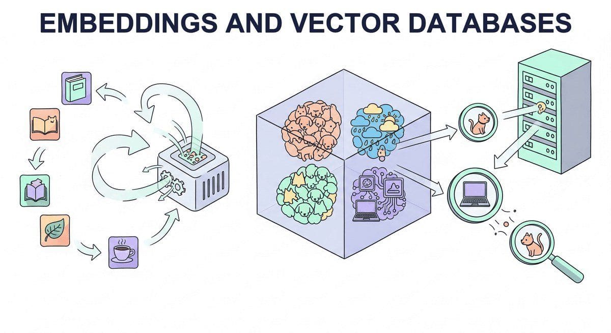
Part VI gave the model agency. Part VII gives it memory. This chapter is the foundation: embeddings (how text becomes vectors), vector databases (how vectors become searchable), and semantic search (how the two combine into "find the most relevant chunk for this query"). Everything in Chapter 32 (RAG), Chapter 33 (Multimodal RAG), and Chapter 37 (Conversational AI) sits on this layer.
Chapter Overview
The sentence "the bank approved the loan" and the sentence "the river bank flooded" share five tokens, but a good embedding model places them on opposite sides of a 1024-dimensional space. That geometry is the engine of every modern search bar, every RAG pipeline, and every "ask your PDF" product launched since 2023. This chapter is about how text becomes vectors (embedding models from Sentence-BERT to OpenAI text-embedding-3 to Voyage and BGE-M3), how those vectors stay searchable at billion-row scale (HNSW, IVF, Product Quantization), and which of the seven vector databases on the 2026 short list actually fits your deployment.
This chapter provides a comprehensive, bottom-up treatment of these foundational components. It begins with the theory and practice of text embedding models, covering the evolution from word-level embeddings to modern sentence transformers and the training objectives that produce high-quality representations. It then examines the data structures and algorithms that make approximate nearest neighbor search practical at scale, including HNSW graphs, inverted file indexes, and product quantization (techniques that parallel the optimization strategies used in LLM inference).
The chapter proceeds to survey the rapidly growing ecosystem of vector database systems, comparing purpose-built solutions like Pinecone, Weaviate, and Qdrant with library-based approaches such as FAISS and embedded databases like ChromaDB. Finally, it addresses the critical (and often overlooked) challenge of document processing and chunking, where poor design decisions can undermine even the most sophisticated retrieval infrastructure.
By the end of this chapter, you will be able to select and fine-tune embedding models for specific domains, design vector indexes that balance recall with latency, deploy and operate vector database systems in production applications, and build document processing pipelines that maximize retrieval quality.
Embeddings transform text into dense vectors that capture semantic meaning, and vector databases make those vectors searchable at scale. This chapter provides the retrieval infrastructure that powers RAG systems in Chapter 32 and grounds the conversational AI systems in Chapter 37.
- Explain the evolution from word embeddings (Word2Vec, GloVe) to sentence-level embeddings (Sentence-BERT, E5, GTE)
- Describe contrastive learning objectives and hard negative mining strategies for training embedding models (building on the transformer encoder architecture)
- Compare cosine similarity, dot product, and Euclidean distance as vector similarity metrics
- Explain HNSW graph construction and search, IVF partitioning, and Product Quantization at a technical level
- Evaluate vector database systems (Pinecone, Weaviate, Qdrant, Milvus, ChromaDB, pgvector) for different deployment scenarios
- Implement hybrid search combining dense vector retrieval with sparse keyword matching using reciprocal rank fusion
- Design document chunking strategies (fixed-size, recursive, semantic, structure-aware) appropriate for different content types, informed by tokenization mechanics
- Build end-to-end RAG ETL pipelines with document loading, parsing, chunking, embedding, and indexing
- Use MTEB benchmarks and custom evaluation sets to select embedding models for specific domains
- Implement incremental indexing and document versioning for production vector search systems
Prerequisites
- Chapter 1: NLP & Text Representation (vector spaces, similarity metrics)
- Chapter 3: The Transformer Architecture (attention, encoder vs. decoder models)
- Chapter 11: LLM APIs (working with embedding API endpoints)
- Comfortable with Python, NumPy, and basic data structures (graphs, hash tables, trees)
- Familiarity with database concepts (indexing, queries, CRUD operations)
Sections
- 31.1 Classical Embedding Foundations From word vectors to sentence-BERT; bi-encoder vs. cross-encoder; pooling strategies; contrastive learning with InfoNCE and hard-negative mining. Entry
- 31.2 Modern Embedding Architectures & Selection Matryoshka representation learning, ColBERT late interaction, the 2024-26 embedding ecosystem, MTEB selection, fine-tuning, and production considerations. Intermediate
- 31.3 ANN Search: HNSW and IVF The nearest neighbor problem, HNSW graphs, and IVF inverted file indexes. Advanced
- 31.4 Product Quantization, Composite Indexes, and FAISS Product quantization, composite indexes, index selection guidance, and the FAISS index factory. Advanced
- 31.5 Vector Database Systems A vector database is more than an ANN index with an API. Intermediate
- 31.6 Document Processing & Chunking The quality of your RAG system is bounded by the quality of your chunks. Advanced
- 31.7 Production RAG Pipelines, Evaluation & Topic Modeling Incremental indexing, metadata enrichment, chunking evaluation against retrieval metrics, and BERTopic topic discovery from the same embeddings. Advanced
- 31.8 Vision-Based Document Retrieval Traditional document retrieval is like a librarian who can only search a typed index of keywords. Advanced
Objective
Pick a retrieval task you actually care about (Stack Overflow Q&A, ArXiv abstracts, your team's docs) and benchmark five embedding models head-to-head on recall@10. By the end you will have a justified embedding choice plus the harness to re-run it whenever a new model drops.
Steps
- Step 1: Build a labeled set. Collect 200 queries with at least one known-correct document (Stack Overflow questions paired with accepted answers work well). Save as
eval.jsonl:{"query":..., "correct_doc_ids":[...]}. - Step 2: Index five embedders. Encode the document corpus with:
text-embedding-3-small,text-embedding-3-large,BAAI/bge-base-en-v1.5,jinaai/jina-embeddings-v3,voyage-3. Persist five FAISS indices. - Step 3: Evaluate. For each model, run all 200 queries, retrieve top-10, compute recall@1, recall@10, MRR. Render as a Markdown table.
- Step 4: Add BM25. Build a sparse index with
rank_bm25. Measure same metrics. Note: BM25 often wins on keyword-heavy queries; dense wins on paraphrase. - Step 5: Hybrid. Combine BM25 + best dense via reciprocal rank fusion (k=60). Measure recall again. Hybrid usually wins by 5 to 10 points.
- Step 6: Cost / latency tradeoff. For each model, record encoding throughput (docs/sec) and per-query latency. Plot recall@10 vs. cost-per-million-queries. Pick a recommended model for production and justify in 3 sentences.
Expected Output
Expected time: 2 to 3 hours. Difficulty: beginner-to-intermediate. Artifact: a benchmark table you can re-run on any new embedder.
What's Next?
Next: Chapter 32: RAG Fundamentals. Embeddings and vector databases give you the substrate. RAG is the pattern that makes them earn their keep. Chapter 32 walks through the full pipeline (chunking strategies that survive contact with real documents, hybrid retrieval, re-ranking, prompt assembly, source attribution and citation) and explains why naive RAG so often fails the moment you try to scale past 1,000 documents.