A chunk is not a deliverable. A maintained, evaluated, topic-aware index is.
Vec, Pipeline-Minded AI Agent
Section 31.4 established how to chunk a document well. This continuation answers what comes after the first batch run: how to keep an index fresh as documents change (incremental indexing, metadata enrichment), how to systematically evaluate chunking choices against retrieval metrics, and how to repurpose the same embeddings into topic models (BERTopic) that surface latent themes in a corpus. Together, these three layers move a chunking strategy from a one-off prototype into a maintained production retrieval system.
Prerequisites
This section continues from Section 31.4: Document Processing & Chunking, which established the chunking strategies (fixed-size, recursive, semantic, structure-aware, parent-child) that this section now operationalizes for production. Familiarity with the embedding model fundamentals in Section 31.1 and the vector database systems in Section 31.5 is assumed.
31.7.1 Production RAG ETL Pipelines
A production ingestion pipeline must handle document updates, deletions, and versioning in addition to initial loading. The key engineering challenges include:
Incremental Indexing
When documents are updated, you must re-chunk and re-embed only the changed documents, not the entire corpus. This requires tracking document versions (typically via content hashes or timestamps) and maintaining a mapping between source documents and their chunks in the vector database.
# Incremental indexing with content hashing
import hashlib
import json
from typing import Dict, List, Optional
from pathlib import Path


class IncrementalIndexer:
    """
    Tracks document versions to enable incremental re-indexing.
    Only processes documents that have changed since the last run.
    """

    def __init__(self, state_file: str = "indexer_state.json"):
        self.state_file = Path(state_file)
        self.state: Dict[str, str] = {}
        if self.state_file.exists():
            self.state = json.loads(self.state_file.read_text())

    def content_hash(self, content: str) -> str:
        return hashlib.sha256(content.encode()).hexdigest()

    def get_changes(
        self, documents: Dict[str, str]
    ) -> Dict[str, List[str]]:
        """
        Compare current documents against stored state.

        Args:
            documents: dict of {doc_id: content}

        Returns:
            {"added": [...], "modified": [...], "deleted": [...]}
        """
        current_ids = set(documents.keys())
        stored_ids = set(self.state.keys())
        added = current_ids - stored_ids
        deleted = stored_ids - current_ids
        modified = set()
        for doc_id in current_ids & stored_ids:
            new_hash = self.content_hash(documents[doc_id])
            if new_hash != self.state[doc_id]:
                modified.add(doc_id)
        return {
            "added": list(added),
            "modified": list(modified),
            "deleted": list(deleted),
        }

    def update_state(self, documents: Dict[str, str]):
        """Update stored hashes after successful indexing."""
        for doc_id, content in documents.items():
            self.state[doc_id] = self.content_hash(content)
        self.state_file.write_text(json.dumps(self.state, indent=2))

    def process_changes(self, documents: Dict[str, str]):
        """Main entry point for incremental processing."""
        changes = self.get_changes(documents)
        print(f"Added: {len(changes['added'])} documents")
        print(f"Modified: {len(changes['modified'])} documents")
        print(f"Deleted: {len(changes['deleted'])} documents")
        # For added/modified: chunk, embed, upsert
        to_process = changes["added"] + changes["modified"]
        if to_process:
            print(f"Processing {len(to_process)} documents...")
            # chunk_and_embed(to_process)
            # vector_db.upsert(chunks)
        # For deleted: remove from vector DB
        if changes["deleted"]:
            print(f"Removing {len(changes['deleted'])} documents...")
            # vector_db.delete(filter={"doc_id": {"$in": changes["deleted"]}})
        # For modified: also remove old chunks before upserting new ones
        if changes["modified"]:
            print(f"Replacing chunks for {len(changes['modified'])} documents...")
            # vector_db.delete(filter={"doc_id": {"$in": changes["modified"]}})
            # vector_db.upsert(new_chunks)
        self.update_state(documents)


# Usage
indexer = IncrementalIndexer()
docs = {
    "report_2024.pdf": "Full text of the 2024 report...",
    "manual_v3.pdf": "Updated product manual content...",
    "faq.md": "Frequently asked questions...",
}
indexer.process_changes(docs)Metadata Enrichment
Every chunk should carry metadata that enables effective filtering and attribution. Essential metadata fields include:
- Source: The original file name or URL for citation and deduplication.
- Page/section: Location within the source document for precise references.
- Title hierarchy: Section and subsection headings for contextual understanding.
- Date: Creation or last-modified date for recency filtering.
- Document type: Category labels (policy, FAQ, report, transcript) for scoped search.
- Access permissions: User or group identifiers for access-controlled retrieval.
The most common mistakes in document processing are: (1) Not evaluating chunking quality by measuring retrieval performance with different strategies and parameters on representative queries. (2) Ignoring document structure by applying the same chunking strategy to all document types. (3) Losing metadata context by stripping headers, section titles, or table captions during chunking. (4) Using the default settings of your framework without tuning chunk size and overlap for your specific content and queries. (5) Not handling tables and figures as special elements that should either be kept intact or described textually.
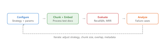
31.7.2 Evaluation and Iteration
Chunking is not a one-time configuration; it requires ongoing evaluation and tuning. The most effective approach is to build a small evaluation set of 50 to 100 representative queries with known relevant passages, then measure retrieval metrics (recall@k, MRR, NDCG) across different chunking configurations. Systematic A/B testing of chunking strategies often reveals that the optimal configuration depends heavily on the document type and query patterns specific to your application. Figure 31.7.1a shows the iterative evaluation loop for chunking quality.
The default HNSW index parameters (ef_construction, M) work for prototyping but not production. Higher ef_construction (256 to 512) improves recall at index build time cost; higher M (32 to 64) improves search quality at memory cost. Tune these based on your recall requirements.
Who: An NLP engineer at a health-tech company building a clinical decision support tool
Situation: The system indexed 120,000 medical journal articles, clinical guidelines, and drug interaction databases. Physicians queried it during patient consultations expecting precise, citation-worthy answers.
Problem: Using a fixed 512-token chunk size produced fragments that split drug dosage tables, broke apart multi-step treatment protocols, and lost critical context about contraindications.
Dilemma: Larger chunks (1,024 tokens) preserved context but reduced retrieval precision because irrelevant content diluted the embedding signal. Smaller chunks (256 tokens) improved precision but often omitted the surrounding clinical context physicians needed.
Decision: The team implemented semantic chunking using section headers and paragraph boundaries, with a target range of 300 to 600 tokens per chunk. They added 2-sentence overlap between adjacent chunks and stored parent document IDs for context expansion at retrieval time.
How: A custom parser detected document structure (headers, lists, tables) and kept logical units intact. Tables were chunked as single units regardless of token count. Metadata (article title, section name, publication year) was prepended to each chunk before embedding.
Result: Answer accuracy (judged by physicians) improved from 71% to 89%. Retrieval precision@5 rose from 0.54 to 0.78, and physicians reported that returned passages were "immediately useful" rather than requiring manual context reconstruction.
Lesson: Chunking strategy should respect document structure rather than applying arbitrary token boundaries. Preserving logical units (tables, protocols, lists) and adding metadata context produces dramatically better retrieval quality.
31.7.3 Topic Modeling with LLM Embeddings
Topic modeling discovers the latent themes in a collection of documents without requiring labeled data. Classical approaches like LDA (Latent Dirichlet Allocation) and NMF (Non-negative Matrix Factorization) operate on bag-of-words representations, which discard word order and semantic nuance. BERTopic (Grootendorst, 2022) replaces this with a pipeline built on the same embedding models used for retrieval, producing topics that are semantically coherent and interpretable. Understanding BERTopic is valuable because the same embeddings you create for RAG (as covered in Section 31.1) can power topic discovery, clustering, and content organization without additional model training.
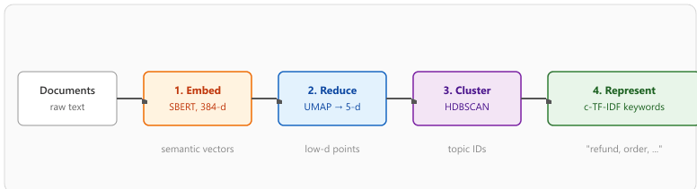
31.7.3.1 The BERTopic Pipeline
BERTopic operates in four sequential stages, each handled by a separate, swappable component:
- Embed: Convert each document to a dense vector using a sentence softmax model (the same models from Section 31.1).
- Reduce: Project the high-dimensional embeddings into a lower-dimensional space using UMAP, preserving local neighborhood structure while making clustering feasible.
- Cluster: Group similar documents using HDBSCAN, a density-based clustering algorithm that automatically determines the number of clusters and identifies outliers (documents that do not fit any topic).
- Represent: Label each cluster with descriptive terms using c-TF-IDF (class-based TF-IDF) or, optionally, an LLM that generates human-readable topic labels from the cluster's representative documents.
The labeling stage uses a class-based variant of TF-IDF (Grootendorst, 2022) that treats each cluster as a single super-document. For class $c$ and term $t$, the c-TF-IDF score is:
where $\mathrm{tf}_{t,c}$ is the frequency of term $t$ inside cluster $c$, $\mathrm{tf}_t$ is its frequency across the whole corpus, and $A$ is the average number of words per cluster. The $\log(1 + A/\mathrm{tf}_t)$ factor penalizes terms that appear everywhere (stopwords) and rewards terms that are concentrated inside one cluster. Sorting terms by c-TF-IDF and keeping the top 10 gives the keyword label that BERTopic reports.
A SaaS company runs BERTopic on 500 customer-support tickets. The four stages produce:
- Embed.
all-MiniLM-L6-v2turns each ticket (avg 28 words) into a 384-d vector. Wall-clock: 4 s on a CPU. - Reduce. UMAP with
n_neighbors=15, n_components=5maps the 384-d vectors into a 5-d space that preserves local neighborhoods. Wall-clock: 6 s. - Cluster. HDBSCAN with
min_cluster_size=15discovers 7 topics plus 42 noise points (8% of the corpus that does not fit any topic). - Represent. c-TF-IDF labels the topics. Topic 0 (123 tickets): "refund, charged, twice, payment, billing". Topic 1 (87 tickets): "password, reset, login, dashboard, email". Topic 2 (61 tickets): "export, csv, download, data, format".
The same five-keyword summary that would have taken a human analyst a full afternoon to produce arrives in under 15 seconds. Re-running with an LLM representation_model upgrades the keyword lists to readable names ("Billing and Refunds", "Account Access", "Data Export").
HDBSCAN clusters by density rather than by a preset cluster count. It first reweights distances into a 'mutual reachability' metric that pushes sparse points apart, then builds a minimum spanning tree and cuts it into a hierarchy of nested clusters at every density threshold. Instead of slicing that hierarchy at one fixed level, it selects the clusters that persist over the widest range of densities, a stability criterion that automatically yields a sensible number of clusters of varying size. Points that never join a dense-enough group are labeled noise rather than forced into a topic. This is why BERTopic discovers topic count on its own and cleanly sets aside off-topic documents that LDA would still assign.
31.7.3.2 BERTopic vs. Classical Topic Models
| Dimension | LDA | NMF | BERTopic |
|---|---|---|---|
| Input representation | Bag-of-words (BoW) | TF-IDF matrix | Dense embeddings (sentence transformers) |
| Semantic awareness | None (word co-occurrence only) | Minimal (term weighting) | Full (contextual embeddings) |
| Number of topics | Must be specified upfront | Must be specified upfront | Automatically determined by HDBSCAN |
| Short text handling | Poor (sparse BoW vectors) | Poor | Good (dense embeddings capture meaning) |
| Topic coherence | Moderate | Good | Excellent (semantically grouped) |
| Scalability | Good (efficient inference) | Good | Moderate (embedding step is the bottleneck) |
| Dynamic topics | Not natively supported | Not natively supported | Built-in support for topics over time |
31.7.3.3 Practical Example
This snippet demonstrates a practical hybrid search query that combines dense and sparse retrieval.
# BERTopic: embedding-based topic modeling
# Uses the same sentence transformers as RAG embedding pipelines
from bertopic import BERTopic
from sentence_transformers import SentenceTransformer
from umap import UMAP
from hdbscan import HDBSCAN
# Step 1: Configure each pipeline component
embedding_model = SentenceTransformer("all-MiniLM-L6-v2")
umap_model = UMAP(
    n_neighbors=15, n_components=5,
    min_dist=0.0, metric="cosine",
    )
hdbscan_model = HDBSCAN(
    min_cluster_size=15,
    metric="euclidean",
    prediction_data=True,
    )
# Step 2: Build the BERTopic model with custom components
topic_model = BERTopic(
    embedding_model=embedding_model,
    umap_model=umap_model,
    hdbscan_model=hdbscan_model,
    verbose=True,
    )
# Step 3: Fit on your documents (e.g., customer support tickets)
documents = [
    "My order has not arrived after two weeks",
    "How do I reset my password for the dashboard?",
    "The API returns a 500 error on large payloads",
    "I was charged twice for the same subscription",
    "Can I export my data as a CSV file?",
    # ... thousands more documents
    ]
topics, probs = topic_model.fit_transform(documents)
# Step 4: Inspect discovered topics
topic_info = topic_model.get_topic_info()
print(topic_info.head(10))
# Step 5: Get the top terms for a specific topic
for topic_id in range(min(5, len(topic_model.get_topics()))):
    terms = topic_model.get_topic(topic_id)
    print(f"\nTopic {topic_id}:")
    for term, score in terms[:5]:
print(f" {score:.3f} {term}")Embedding-based topic models like BERTopic outperform bag-of-words approaches (LDA, NMF) because they capture semantic similarity rather than surface-level word co-occurrence. Two documents about "machine learning model deployment" and "putting ML systems into production" share no words in common, so LDA would assign them to different topics. BERTopic, working from dense embeddings, recognizes they discuss the same concept and clusters them together. This semantic awareness is especially valuable for short texts (tweets, support tickets, search queries) where bag-of-words vectors are too sparse to produce meaningful topics.
BERTopic can optionally use an LLM to generate human-readable topic labels. Instead of a topic being described as "deployment, production, inference, serving, latency," the LLM reads the cluster's representative documents and produces a label like "ML Model Deployment and Serving Infrastructure." This makes topic models immediately useful for non-technical stakeholders who need to understand what their customer base is talking about.
31.7.3.4 Plug-In Representation Models
The default c-TF-IDF keyword list per topic is a reasonable starting point but rarely the most readable one. BERTopic exposes a representation_model hook so the four-stage pipeline (embed, reduce, cluster, represent) can be customized at the final step without touching the upstream UMAP or HDBSCAN configuration. Three plug-ins cover almost every production need.
KeyBERTInspired re-ranks the top c-TF-IDF candidate words for each topic by their cosine similarity to the topic's centroid embedding. The intuition is that c-TF-IDF favors words that distinguish the cluster from other clusters statistically, but those words are not always the words a human would call descriptive. KeyBERTInspired pushes the keyword list toward terms that are semantically central to the topic, not just statistically distinctive. MaximalMarginalRelevance applies the MMR algorithm (see Section 35.2.1.5) to the candidate keywords, so the final list trades relevance against diversity and avoids near-duplicates like "summary" and "summaries" both surfacing for the same topic. OpenAI hands a few representative documents per topic to an LLM and asks it to write a one-line topic label, the same trick promised in the fun-fact above but now an actual line of code. The three plug-ins stack:
from bertopic import BERTopic
from bertopic.representation import (
    KeyBERTInspired, MaximalMarginalRelevance, OpenAI,
)
from openai import OpenAI as OpenAIClient

client = OpenAIClient()

representation = {
    "Main":      KeyBERTInspired(),                          # centroid-aware keywords
    "MMR":       MaximalMarginalRelevance(diversity=0.3),    # de-duped keywords
    "LLM Label": OpenAI(client=client, model="gpt-4o-mini"), # one-line topic name
}

topic_model = BERTopic(
    embedding_model=embedder,
    representation_model=representation,
)
topics, _ = topic_model.fit_transform(docs)
print(topic_model.get_topic_info().head())get_topic_info(), so a downstream UI can display the LLM label, fall back to the KeyBERT keywords, and use the MMR list for tag clouds without rerunning UMAP or HDBSCAN.31.7.3.5 BERTopic Visualizations
BERTopic ships an interactive visualization layer that turns the topic model into a quick analytical UI without writing any plotting code. Four methods cover the common reporting needs: visualize_documents() plots every document as a point in 2-D UMAP space, colored by topic, with hover tooltips showing the document text; visualize_topics() draws an inter-topic distance map so reviewers can see which topics overlap and which are well separated; visualize_hierarchy() renders the dendrogram of agglomerative clustering over topic embeddings, which is the input to the next method; reduce_topics(nr_topics=20) collapses fine-grained topics into a target number using that same hierarchy, useful when HDBSCAN produces 80 small topics but the business audience wants 10 broad themes. All four return Plotly figures that drop directly into a Jupyter notebook or a Streamlit dashboard.
LLM-guided chunking uses language models to identify semantic boundaries in documents, producing chunks that align with topical shifts rather than arbitrary token counts. Late chunking (Jina AI, 2024) embeds the full document first and then splits the embedding sequence into chunks, preserving cross-chunk context that is lost with naive chunking. Proposition-based indexing decomposes documents into atomic factual statements before embedding, improving retrieval precision for fact-seeking queries. Research into multimodal document parsing (combining OCR, layout analysis, and vision models) is enabling chunking of complex documents with tables, figures, and mixed layouts.
Objective
Implement three different chunking strategies (fixed-size, recursive, semantic), apply them to a structured document, and compare their retrieval quality on test queries.
What You'll Practice
- Implementing fixed-size chunking with character-based overlap
- Building recursive text splitting using structural markers (headers, paragraphs)
- Creating semantic chunking using embedding similarity breakpoints
- Measuring retrieval quality differences between chunking strategies
Setup
The following cell installs the required packages and configures the environment for this lab.
Steps
Step 1: Create a sample document
Define a structured document with clear section boundaries.
document = (
    "# Introduction to Machine Learning\n\n"
    "Machine learning is a branch of artificial intelligence that enables "
    "computers to learn from data without being explicitly programmed.\n\n"
    "## Supervised Learning\n\n"
    "In supervised learning, the algorithm learns from labeled training data. "
    "Each example consists of an input and a desired output.\n\n"
    "### Classification\n\n"
    "Classification predicts categorical labels. For example, an email spam "
    "filter classifies emails as spam or not spam. Popular algorithms include "
    "logistic regression, SVMs, and random forests.\n\n"
    "### Regression\n\n"
    "Regression predicts continuous numerical values. For instance, predicting "
    "house prices based on features like square footage and location.\n\n"
    "## Unsupervised Learning\n\n"
    "Unsupervised learning works with unlabeled data, seeking to discover "
    "hidden patterns and structures without target labels.\n\n"
    "### Clustering\n\n"
    "Clustering groups similar data points together. K-means partitions data "
    "into k groups. DBSCAN discovers clusters of arbitrary shape based on "
    "density. Hierarchical clustering builds a tree of nested clusters.\n\n"
    "### Dimensionality Reduction\n\n"
    "Dimensionality reduction compresses high-dimensional data. PCA finds "
    "directions of maximum variance. t-SNE and UMAP create 2D visualizations "
    "that preserve local neighborhood structure.\n\n"
    "## Deep Learning\n\n"
    "Deep learning uses neural networks with many layers to learn hierarchical "
    "representations. It has achieved breakthroughs in vision, NLP, and games."
)
print(f"Document: {len(document)} chars, {document.count(chr(10))} lines")Hint
This document has clear structural markers: # for h1, ## for h2, ### for h3, and blank lines between paragraphs. Good chunking should respect these boundaries.
Step 2: Implement three chunking strategies
Build fixed-size, recursive, and semantic chunkers.
import numpy as np
from sentence_transformers import SentenceTransformer
model = SentenceTransformer("all-MiniLM-L6-v2")
# Strategy 1: Fixed-size with overlap
def fixed_chunk(text, size=300, overlap=50):
    chunks, start = [], 0
    while start < len(text):
        chunk = text[start:start+size].strip()
        if chunk:
            chunks.append(chunk)
            start += size - overlap
            return chunks
# Strategy 2: Recursive splitting on headers
def recursive_chunk(text, max_size=500):
    # TODO: Split on "## " first, then "### " for oversized sections
    # Merge chunks smaller than max_size/3 with their neighbors
    sections = text.split("\n## ")
    chunks = []
    for section in sections:
        section = section.strip()
        if not section:
            continue
        if len(section) <= max_size:
            chunks.append(section)
        else:
            for sub in section.split("\n### "):
                sub = sub.strip()
                if sub:
                    chunks.append(sub)
                    return chunks
# Strategy 3: Semantic chunking
def semantic_chunk(text, model, threshold=0.5):
    # TODO: Split into sentences, encode them, find similarity drops
    sentences = [s.strip() for s in text.replace('\n', ' ').split('. ')
        if len(s.strip()) > 10]
    if len(sentences) <= 1:
        return sentences
    embs = model.encode(sentences)
    norms = np.linalg.norm(embs, axis=1)
    chunks, current = [], [sentences[0]]
    for i in range(len(sentences) - 1):
        sim = np.dot(embs[i], embs[i+1]) / (norms[i] * norms[i+1] + 1e-8)
        if sim < threshold:
            chunks.append(". ".join(current))
            current = [sentences[i+1]]
        else:
            current.append(sentences[i+1])
            if current:
                chunks.append(". ".join(current))
                return chunks
            c_fixed = fixed_chunk(document)
            c_recursive = recursive_chunk(document)
            c_semantic = semantic_chunk(document, model)
            for name, chunks in [("Fixed", c_fixed), ("Recursive", c_recursive),
                ("Semantic", c_semantic)]:
                print(f"\n{name}: {len(chunks)} chunks")
                for i, c in enumerate(chunks):
print(f" [{i}] {len(c)} chars: {c[:60]}...")Hint
For semantic chunking, compute cosine similarity between consecutive sentence embeddings. A drop below the threshold signals a topic change, which is where you create a new chunk.
Step 3: Compare retrieval quality
Search each set of chunks and check which strategy finds the best match.
import numpy as np
queries_expected = [
    ("What is classification in ML?", "classification"),
    ("How does clustering work?", "clustering"),
    ("What is PCA used for?", "dimensionality"),
    ("What is deep learning?", "deep learning"),
    ]
def search_chunks(query, chunks, model, top_k=1):
    qe = model.encode(query)
    ce = model.encode(chunks)
    scores = np.dot(ce, qe) / (np.linalg.norm(ce, axis=1) * np.linalg.norm(qe))
    idx = np.argsort(scores)[::-1][:top_k]
    return [(chunks[i], scores[i]) for i in idx]
for query, keyword in queries_expected:
    print(f"\nQuery: {query}")
    for name, chunks in [("Fixed", c_fixed), ("Recursive", c_recursive),
        ("Semantic", c_semantic)]:
        top_chunk, score = search_chunks(query, chunks, model)[0]
        hit = "PASS" if keyword.lower() in top_chunk.lower() else "MISS"
        print(f" {name:10s} [{hit}] score={score:.3f} | {top_chunk[:55]}...")
Hint
Recursive chunking should perform best because chunks align with natural topic boundaries. Fixed-size chunks may split topics mid-sentence.
Expected Output
- Three sets of chunks with different sizes (fixed: ~8, recursive: ~6, semantic: ~5 to 8)
- Recursive and semantic chunking matching relevant chunks more reliably
- Fixed-size chunking occasionally missing because topics get split at boundaries
Stretch Goals
- Add metadata (section title, position) to each chunk and use it to improve retrieval context
- Implement a "parent document retriever" that returns the larger parent section when a small chunk matches
- Test on a real PDF by extracting text with PyMuPDF and applying the same strategies
Complete Solution
import numpy as np
from sentence_transformers import SentenceTransformer
model = SentenceTransformer("all-MiniLM-L6-v2")
document = (
    "# Introduction to Machine Learning\n\n"
    "Machine learning enables computers to learn from data.\n\n"
    "## Supervised Learning\n\nLearns from labeled data.\n\n"
    "### Classification\n\nPredicts categorical labels like spam/not-spam.\n\n"
    "### Regression\n\nPredicts continuous values like house prices.\n\n"
    "## Unsupervised Learning\n\nFinds patterns in unlabeled data.\n\n"
    "### Clustering\n\nGroups similar points. K-means, DBSCAN, hierarchical.\n\n"
    "### Dimensionality Reduction\n\nCompresses data. PCA, t-SNE, UMAP.\n\n"
    "## Deep Learning\n\nNeural networks with many layers for hierarchical representations."
    )
def fixed_chunk(text, size=300, overlap=50):
    chunks, s = [], 0
    while s < len(text):
        c = text[s:s+size].strip()
        if c: chunks.append(c)
        s += size - overlap
        return chunks
def recursive_chunk(text, max_size=500):
    chunks = []
    for sec in text.split("\n## "):
        sec = sec.strip()
        if not sec: continue
        if len(sec) <= max_size: chunks.append(sec)
    else:
        for sub in sec.split("\n### "):
            sub = sub.strip()
            if sub: chunks.append(sub)
            return chunks
def semantic_chunk(text, model, threshold=0.5):
    sents = [s.strip() for s in text.replace('\n',' ').split('. ') if len(s.strip())>10]
    if len(sents) <= 1: return sents
    embs = model.encode(sents)
    norms = np.linalg.norm(embs, axis=1)
    chunks, cur = [], [sents[0]]
    for i in range(len(sents)-1):
        sim = np.dot(embs[i],embs[i+1])/(norms[i]*norms[i+1]+1e-8)
        if sim < threshold: chunks.append(". ".join(cur)); cur = [sents[i+1]]
    else: cur.append(sents[i+1])
    if cur: chunks.append(". ".join(cur))
    return chunks
cf, cr, cs = fixed_chunk(document), recursive_chunk(document), semantic_chunk(document, model)
def search(q, chunks, model):
    qe = model.encode(q); ce = model.encode(chunks)
    scores = np.dot(ce,qe)/(np.linalg.norm(ce,axis=1)*np.linalg.norm(qe))
    i = np.argmax(scores)
    return chunks[i], scores[i]
for q, kw in [("What is classification?","classification"),("How does clustering work?","clustering"),
    ("What is PCA?","dimensionality"),("What is deep learning?","deep learning")]:
    print(f"\n{q}")
    for nm, ch in [("Fixed",cf),("Recursive",cr),("Semantic",cs)]:
        c, s = search(q, ch, model)
print(f" {nm:10s} [{'PASS' if kw in c.lower() else 'MISS'}] {s:.3f} | {c[:55]}")The hand-rolled np.dot / np.linalg.norm loop above shows the math; the library version is what you would ship. In production, prefer sklearn.metrics.pairwise.cosine_similarity(A, B) (vectorized over arrays, drop-in replacement for the loop above) for moderate corpora, or faiss.IndexFlatIP with L2-normalized vectors when you need billion-scale retrieval. See the next two Library Shortcut blocks for ready-to-paste sklearn and LangChain wrappers.
Reach for sklearn when you need a one-call cosine search over a moderate corpus. For larger indexes, swap in FAISS the same way as in Section 31.2.
Show code
from sklearn.metrics.pairwise import cosine_similarity
import numpy as np

def search_chunks(query, chunks, model, top_k=1):
    qe = model.encode([query])
    ce = model.encode(chunks)
    sims = cosine_similarity(qe, ce)[0]
    idx = np.argsort(sims)[::-1][:top_k]
return [(chunks[i], sims[i]) for i in idx]search_chunks() helper that embeds both the query and the candidate chunks on the fly, then uses sklearn.cosine_similarity to return the best-matching chunk and its score (handy for one-off retrieval without a persistent index).LangChain ships a battle-tested splitter that handles the recursive fallback (paragraph → sentence → word) and overlap in a single call. Production RAG pipelines almost always use this.
Show code
from langchain_text_splitters import RecursiveCharacterTextSplitter

splitter = RecursiveCharacterTextSplitter(
    chunk_size=500, chunk_overlap=50,
    separators=["\n## ", "\n### ", "\n\n", "\n", ". ", " "],
)
chunks = splitter.split_text(document)LangChain RecursiveCharacterTextSplitter.- Chunking quality bounds RAG quality. No downstream component can compensate for chunks that split relevant information or mix unrelated topics.
- Recursive character splitting is the best default for most text content, balancing simplicity with respect for natural text boundaries.
- Semantic chunking produces the most coherent chunks by detecting topic boundaries via embedding similarity, at the cost of additional computation.
- Structure-aware chunking is essential for formatted documents (PDFs, HTML, Markdown) where headings, tables, and figures define natural semantic units.
- Parent-child retrieval resolves the chunk-size tradeoff by using small chunks for precise retrieval and large chunks for LLM context.
- Always enrich chunks with metadata (source, page, section title, date) to enable filtered search and proper attribution.
- Build an evaluation set of representative queries with known relevant passages, and systematically test chunking configurations against retrieval metrics.
- Incremental indexing with content hashing is essential for production pipelines that process evolving document collections.
Show Answer
Show Answer
Show Answer
Show Answer
Show Answer
Exercises
A 200-token chunk about climate change is highly precise for retrieval, but the LLM struggles to generate a good answer from it. A 1000-token chunk provides more context but retrieves poorly. How would you resolve this tension?
Show Answer
Use parent-child retrieval: embed small chunks (200 tokens) for precise retrieval, but pass the larger parent chunk (800 to 1000 tokens) to the LLM for generation. This gets the best of both worlds.
Explain why overlapping chunks improve retrieval quality. What percentage of overlap is typical, and what happens if overlap is too high?
Show Answer
Overlap ensures that information spanning a chunk boundary is captured in at least one chunk. Typical overlap is 10 to 15% of chunk size. Excessive overlap (e.g., 50%) wastes storage and creates near-duplicate embeddings that dilute search results.
Compare fixed-size chunking with semantic chunking (splitting at topic boundaries). When does semantic chunking clearly outperform fixed-size, and when is fixed-size good enough?
Show Answer
Semantic chunking outperforms fixed-size when documents contain clear topic shifts (e.g., news articles, textbooks). Fixed-size is good enough when documents are homogeneous (e.g., product reviews, FAQ entries) or when the retrieval pipeline includes reranking.
Describe the parent-child chunking strategy. Why would you retrieve on small chunks but pass the parent chunk to the LLM?
Show Answer
Small child chunks produce more focused embeddings (better retrieval precision), while parent chunks give the LLM enough surrounding context to generate coherent, grounded answers.
You have a 200-page financial report with charts, tables, and prose. Compare two approaches: (a) extract text only and chunk, (b) use vision-based retrieval with ColPali. What are the tradeoffs?
Show Answer
(a) Text extraction loses visual layout, table structure, and chart data, but is faster and cheaper. (b) ColPali preserves visual information and handles charts/tables natively, but requires more compute and storage (one embedding per page patch). Best approach: use text extraction for prose-heavy sections and ColPali for pages with visual elements.
Take a 5-page document and chunk it three ways: fixed 512 tokens, recursive character splitting, and by paragraph boundaries. Count the chunks produced and examine where splits occur. Which method preserves semantic coherence best?
Write an evaluation script: given a set of 20 questions with known answer passages, embed all chunks using a sentence transformer, retrieve top-5 for each question, and compute Hit Rate and MRR. Compare across chunk sizes of 128, 256, 512, and 1024 tokens.
Use BERTopic on a collection of at least 500 documents (e.g., 20 Newsgroups). Visualize the discovered topics and compare them against the known categories.
Implement a parent-child retrieval system where child chunks (128 tokens) are used for retrieval but parent chunks (512 tokens) are passed to the LLM. Compare answer quality against a flat 512-token chunking approach.
What Comes Next
In the next section, Section 31.8: Vision-Based Document Retrieval, we explore how vision-based retrieval with ColPali and ColQwen2 bypasses the text extraction pipeline entirely by processing document pages as images, enabling retrieval from visually rich content that text-based methods cannot handle.