A model that claims to read a novel but forgets the first chapter by the last page has a context window in name only.
Eval, Forgetfully Long-Context AI Agent
The "context length" listed on a model card is a theoretical maximum, not a guarantee of effective utilization. A 128K token window loses real accuracy on information placed in the middle of a long document, the "lost-in-the-middle" effect documented in Section 32.1. This section covers benchmarks that measure real context utilization (LongBench v2, RULER, Needle-in-a-Haystack), methods that extend context windows past training-time limits (YaRN, NTK-aware scaling, position interpolation), and the evaluation pitfalls that make long-context assessment harder than it looks. For practitioners building RAG systems, effective context length decides the architecture: rely on a long-context model when retrieval can keep up, fall back to RAG when it cannot.
Prerequisites
This section builds on the evaluation fundamentals from Section 42.1 and the experimental design principles in Section 42.2. Understanding positional encoding and attention mechanisms from the Transformer architecture chapter will help with the context extension methods. Familiarity with inference optimization provides useful context for the computational aspects of long-context processing.
42.8.1 The Gap Between Claimed and Effective Context Length
When a model provider advertises a 128K or 1M token context window, that number represents the maximum sequence length the model can accept as input. It does not guarantee that the model will accurately attend to, reason about, or recall information at every position within that window. Several factors contribute to degraded performance at long context lengths:
- Attention dilution: As sequence length grows, attention weights spread across more tokens. Information at positions that receive low attention scores is effectively invisible to the model, even though it is technically within the context window.
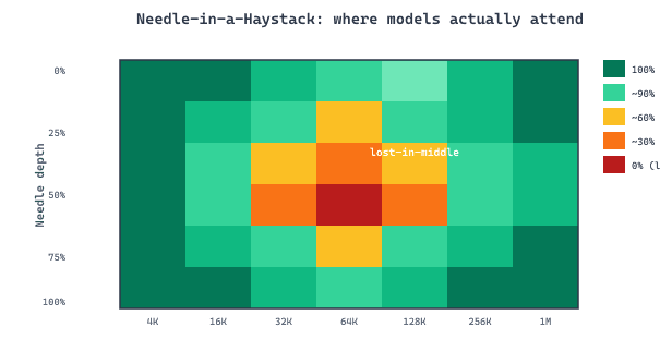
- Position bias: Models trained predominantly on shorter sequences develop a bias toward information near the beginning and end of the context, with reduced recall for content in the middle. This is the "lost-in-the-middle" phenomenon documented by Liu et al. (2023).
- Training distribution mismatch: If a model was pretrained on 4K token sequences and then extended to 128K through positional extrapolation, its ability to reason over the extended range may be significantly weaker than at the original training length.
- Task complexity interaction: Simple retrieval (finding a specific fact) degrades more gracefully than complex reasoning (synthesizing information from multiple positions) as context grows.
The practical consequence: stuffing 100K tokens into a prompt routinely produces worse answers than carefully selecting 10K tokens of relevant content. The wider you spread the model's attention, the thinner the signal at the position you actually care about. Benchmarks in the following sections measure this gap empirically.
Before choosing between a long-context model and a RAG pipeline, run a Needle-in-a-Haystack test at your target context length. If the model drops below 90% retrieval accuracy in the middle third of the context window, you are better off using RAG to select the most relevant chunks than relying on the model to find the information itself.
42.8.2 Needle-in-a-Haystack (NIAH) and Multi-Needle Variants
The Needle-in-a-Haystack (NIAH) test, popularized by Greg Kamradt in late 2023, is the simplest and most intuitive long-context benchmark. A synthetic "needle" (a specific fact, such as "The best thing to do in San Francisco is eat a sandwich and sit in Dolores Park on a sunny day") is inserted at a controlled position within a large "haystack" of irrelevant text. The model is then asked to retrieve the needle.
By varying both the total context length and the needle position (from 0% to 100% depth), NIAH produces a two-dimensional heatmap showing retrieval accuracy across the entire context window. This reveals position-dependent failure patterns that a single aggregate accuracy number would hide.
42.8.2.1 Multi-Needle and Reasoning Variants
The basic single-needle test has been extended in several ways to increase difficulty:
- Multi-needle: Multiple facts are scattered throughout the context, and the model must retrieve all of them. This tests whether the model can attend to multiple positions simultaneously.
- Reasoning needles: Instead of retrieving a verbatim fact, the model must combine information from two or more needles placed at different positions to produce the correct answer.
- Adversarial needles: Distractor facts similar to the target needle are inserted at other positions, testing whether the model can distinguish the correct needle from plausible alternatives.
import numpy as np
from openai import OpenAI
client = OpenAI()
def run_niah_test(
    model: str,
    context_lengths: list[int],
    depth_percents: list[float],
    needle: str = "The secret project code name is AURORA-7.",
    question: str = "What is the secret project code name?",
    expected: str = "AURORA-7",
    filler_text: str = None,
    ) -> np.ndarray:
    """Run NIAH across context lengths and needle positions."""
    results = np.zeros((len(context_lengths), len(depth_percents)))
    for i, ctx_len in enumerate(context_lengths):
        # Generate filler text to fill the context
        haystack = generate_filler(ctx_len, filler_text)
        for j, depth in enumerate(depth_percents):
            # Insert needle at the specified depth
            insert_pos = int(len(haystack) * depth)
            prompt = (
                haystack[:insert_pos]
                + f"\n{needle}\n"
                + haystack[insert_pos:]
                )
            response = client.chat.completions.create(
                model=model,
                messages=[
                {"role": "system",
                "content": "Answer based on the provided context."},
                {"role": "user",
                "content": f"Context:\n{prompt}\n\n{question}"},
                ],
                max_tokens=50,
                temperature=0.0,
                )
            answer = response.choices[0].message.content
            results[i, j] = 1.0 if expected.lower() in answer.lower() else 0.0
            return results
            # Run across multiple context lengths and positions
            context_lengths = [1_000, 4_000, 16_000, 32_000, 64_000, 128_000]
            depth_percents = [0.0, 0.1, 0.25, 0.5, 0.75, 0.9, 1.0]
            scores = run_niah_test(
                model="gpt-4o",
                context_lengths=context_lengths,
                depth_percents=depth_percents,
                )
print(f"Overall retrieval accuracy: {scores.mean():.1%}")The same result in 8 lines with Inspect AI, which ships with a built-in NIAH evaluation task:
Show code
# pip install inspect-ai
from inspect_ai import eval
from inspect_ai.dataset import Sample
from inspect_evals.niah import niah
# Run NIAH across context lengths with one call
results = eval(
    niah(min_context=1_000, max_context=128_000, n_contexts=6, n_positions=7),
    model="openai/gpt-4o",
    log_dir="./niah_logs",
)
# Results include a 2D accuracy matrix and interactive log viewerThe original Needle-in-a-Haystack test went viral on Twitter/X in November 2023 when Greg Kamradt published colorful heatmaps showing that Claude 2.1 had a "blind spot" in the middle of its context window. Anthropic responded within days with a system prompt fix that significantly improved mid-context retrieval. The episode demonstrated both the power of simple, visual benchmarks and the surprising sensitivity of LLM performance to system prompt phrasing.
42.8.3 RULER: Parametric Context Utilization Benchmark
RULER (Hsieh et al., 2024) addresses the limitations of NIAH by providing a parametric benchmark with configurable task complexity. While NIAH tests simple retrieval of a single fact, RULER includes tasks that require reasoning, aggregation, and multi-step operations across the context. RULER defines four task categories:
- Retrieval (NIAH variants): Single-key, multi-key, multi-value, and multi-query needle retrieval at controlled positions.
- Multi-hop tracing: Variable-length chains where the model must follow a sequence of references (e.g., "X is stored in Y, Y is stored in Z; where is X?").
- Aggregation: The model must count, sum, or find the most frequent item among values scattered throughout the context.
- Question answering: Complex questions requiring information from multiple context positions.
The key insight of RULER is that model performance degrades at very different rates depending on task complexity. A model that achieves 95% on single-needle retrieval at 128K tokens may drop to 40% on multi-hop tracing at the same length. RULER's parametric design allows benchmarking at any target sequence length, producing "RULER curves" that show how each task type degrades with context.
import random
import string
def generate_ruler_tracing_task(
    context_length: int,
    chain_length: int = 3,
    num_distractors: int = 20,
    ) -> dict:
    """Generate a RULER-style variable-length tracing task.
    Creates a chain: X is in box A, box A is in box B, ...
    The model must determine the final location of X.
    """
    # Generate unique variable names
    names = [
        "".join(random.choices(string.ascii_uppercase, k=4))
        for _ in range(chain_length + 1 + num_distractors)
        ]
    target = names[0]
    chain_locations = names[1:chain_length + 1]
    distractor_names = names[chain_length + 1:]
    # Build the chain statements
    chain_facts = []
    chain_facts.append(
        f"The item '{target}' is stored in container '{chain_locations[0]}'."
        )
    for k in range(len(chain_locations) - 1):
        chain_facts.append(
            f"Container '{chain_locations[k]}' is inside "
            f"container '{chain_locations[k+1]}'."
            )
        # Build distractor statements
        distractor_facts = []
        for name in distractor_names:
            loc = random.choice(distractor_names)
            distractor_facts.append(
                f"The item '{name}' is stored in container '{loc}'."
                )
            # Interleave chain facts at random positions among distractors
            all_facts = distractor_facts.copy()
            for fact in chain_facts:
                pos = random.randint(0, len(all_facts))
                all_facts.insert(pos, fact)
                # Pad to target context length with filler
                context = "\n".join(all_facts)
                context = pad_to_length(context, context_length)
                return {
                    "context": context,
                    "question": f"Where is '{target}' ultimately stored? "
                    f"Follow the chain of containers.",
                    "expected": chain_locations[-1],
                    "chain_length": chain_length,
                    }
                # Evaluate across context lengths and chain depths
                for ctx_len in [4_000, 32_000, 128_000]:
                    for chain_len in [2, 3, 5, 7]:
                        task = generate_ruler_tracing_task(ctx_len, chain_len)
                        result = evaluate_model(task)
                        print(f"Context: {ctx_len:>7,} | Chain: {chain_len} | "
f"Correct: {result}")42.8.4 LongBench v2: Multi-Task Long-Context Evaluation
LongBench v2 (Bai et al., 2024) provides a comprehensive, multi-task evaluation suite for long-context language models. Unlike synthetic benchmarks (NIAH, RULER), LongBench v2 uses real-world documents and tasks that reflect actual long-context use cases. The benchmark spans six task categories:
- Single-document QA: Questions answerable from a single long document (academic papers, legal contracts, technical manuals).
- Multi-document QA: Questions requiring synthesis across multiple documents concatenated into a single context.
- Summarization: Producing summaries of long documents that capture key information without hallucination.
- Few-shot learning: In-context learning with many demonstration examples, testing whether models can leverage large example sets effectively.
- Code completion: Completing code given a large repository context with cross-file dependencies.
- Synthetic tasks: Controlled tasks (including NIAH variants) for isolating specific capabilities.
LongBench v2 addresses several shortcomings of earlier benchmarks. It uses a "length-instruction-enhanced" evaluation protocol that controls for the confound between task difficulty and context length. Tasks are designed so that the relevant information truly requires the full context, preventing models from "cheating" by ignoring the long context and relying on parametric knowledge.
A critical finding from LongBench v2: model rankings flip across task categories and context lengths. The model that leads on single-document QA at 32K tokens ranks last on multi-document synthesis at 128K tokens. A single "long-context score" is therefore misleading. Evaluate on the specific task type and context length that matches your production workload, not on aggregate leaderboard positions.
42.8.5 Context Extension Methods
Models trained with a fixed maximum sequence length face a hard boundary: they cannot process inputs longer than their training context. Positional encoding extension methods address this by modifying the position representation so that the model can generalize to longer sequences without full retraining. The key methods are:
42.8.5.1 Position Interpolation
Position interpolation (Chen et al., 2023) is the simplest extension method. Instead of extrapolating RoPE (Rotary Position Embedding) frequencies beyond the training range, it rescales all positions to fit within the original range. For a model trained on $L$ tokens extended to $L' > L$ tokens, position $i$ is mapped to $i \cdot \frac{L}{L'}$.
The intuition is that interpolation between known positions is more stable than extrapolation beyond them. A model trained on positions 0 through 4,096 can reasonably estimate what position 2,048.5 "looks like," but has no reliable basis for estimating position 8,192. After interpolation, a small amount of fine-tuning (typically 1,000 steps) adapts the model to the compressed position representation.
42.8.5.2 NTK-Aware Scaling
NTK-aware scaling (bloc97, 2023) observes that position interpolation compresses high-frequency RoPE components too aggressively, destroying local position information. Instead of applying a uniform scaling factor, NTK-aware scaling adjusts the RoPE base frequency:
$$\theta'_i = \theta_{\text{base}}^{\prime -2i/d} \quad \text{where} \quad \theta_{\text{base}}' = \theta_{\text{base}} \cdot \alpha^{d/(d-2)}$$Here, $\alpha = L'/L$ is the extension ratio and $d$ is the embedding dimension. This preserves high-frequency (local) positional information while stretching low-frequency (global) components to accommodate longer sequences. NTK-aware scaling often works without any fine-tuning at moderate extension ratios (2x to 4x).
42.8.5.3 YaRN (Yet another RoPE extensioN)
YaRN (Peng et al., 2023) combines the best ideas from position interpolation and NTK-aware scaling into a unified framework. It introduces a per-dimension scaling strategy that treats RoPE frequency bands differently based on their wavelength relative to the original context length:
- High-frequency dimensions (wavelength much shorter than training length): No scaling needed; these encode local position information that transfers directly.
- Low-frequency dimensions (wavelength comparable to or longer than training length): Apply NTK-aware scaling to stretch these for the extended context.
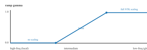
- Intermediate dimensions: Blend between no scaling and full scaling using a smooth ramp function.
YaRN also applies a temperature scaling factor to the attention logits to compensate for the increased entropy of attention distributions at longer sequence lengths. This correction prevents the "attention dilution" that would otherwise degrade performance.
Formally, let $s = L'/L$ be the extension ratio from training length $L$ to target length $L'$, and let $\lambda_i = 2\pi / \theta_i$ be the wavelength of RoPE dimension $i$. YaRN defines a smooth ramp $\gamma(\lambda_i)$ that interpolates between no scaling (high frequencies) and full NTK scaling (low frequencies):
$$\gamma(\lambda_i) = \mathrm{clip}\!\left(\frac{L/\beta_{\text{fast}} - \lambda_i}{L/\beta_{\text{fast}} - L/\beta_{\text{slow}}},\; 0,\; 1\right)$$
The per-dimension scaled frequency is then a blend of the original $\theta_i$ and the NTK-stretched $\theta_i^{\text{NTK}} = \theta_i / s^{d/(d-2)}$:
$$\theta_i^{\text{YaRN}} \;=\; (1 - \gamma(\lambda_i))\, \theta_i \;+\; \gamma(\lambda_i)\, \theta_i^{\text{NTK}} .$$
To counter attention dilution at long sequences, YaRN multiplies attention logits by an inverse temperature $1/t$ with $t = 0.1 \ln(s) + 1$, so the softmax stays sharp even when many more keys compete for probability mass. The rationale follows from the entropy of the attention softmax: when the sequence grows by a factor $s$, the softmax is taken over proportionally more positions, so its entropy rises (attention spreads thinner and the weight on the genuinely relevant key shrinks). Scaling the logits by $1/t$ (equivalently, applying temperature $t$) re-sharpens the distribution and recovers roughly the effective attention concentration the model had at its training length. The logarithmic form $t = 0.1\ln(s) + 1$ mirrors the fact that softmax entropy grows logarithmically with the number of competing positions, so the correction need only grow logarithmically with the extension ratio; at $s = 1$ it reduces to $t = 1$, applying no change, as it must.
The code below implements this ramp directly. Each RoPE frequency is reweighted according to its wavelength relative to the original training length, producing the blended frequencies that YaRN feeds into the attention computation.
import torch
import math
def yarn_rope_scaling(
    dim: int,
    max_position: int,
    original_max: int = 4096,
    base: float = 10000.0,
    beta_fast: int = 32,
    beta_slow: int = 1,
    ) -> torch.Tensor:
    """Compute YaRN-scaled RoPE frequencies.
    Args:
    dim: RoPE embedding dimension
    max_position: target context length
    original_max: original training context length
    base: RoPE base frequency
    beta_fast: fast (high-freq) interpolation boundary
    beta_slow: slow (low-freq) interpolation boundary
    """
    scale = max_position / original_max
    # Compute original frequencies
    freqs = 1.0 / (base ** (torch.arange(0, dim, 2).float() / dim))
    # Compute wavelengths for each frequency dimension
    wavelengths = 2 * math.pi / freqs
    # Determine per-dimension scaling using ramp function
    low_bound = original_max / beta_fast
    high_bound = original_max / beta_slow
    # Ramp: 0 for high-freq (no scaling), 1 for low-freq (full scaling)
    ramp = ((wavelengths - low_bound) / (high_bound - low_bound)).clamp(0, 1)
    # Interpolate between original freqs and NTK-scaled freqs
    ntk_factor = base * (scale ** (dim / (dim - 2)))
    ntk_freqs = 1.0 / (ntk_factor ** (torch.arange(0, dim, 2).float() / dim))
    # Blend: high-freq keeps original, low-freq uses NTK scaling
    scaled_freqs = (1 - ramp) * freqs + ramp * ntk_freqs
    return scaled_freqs
# Example: extend a 4K model to 128K
freqs_4k = yarn_rope_scaling(dim=128, max_position=4096,
    original_max=4096)
freqs_128k = yarn_rope_scaling(dim=128, max_position=131072,
    original_max=4096)
print(f"Scaling ratio: {131072 / 4096}x")
print(f"Low-freq stretch: {freqs_4k[-1] / freqs_128k[-1]:.1f}x")
print(f"High-freq stretch: {freqs_4k[0] / freqs_128k[0]:.1f}x")In practice no one re-implements the ramp by hand; the HuggingFace transformers config exposes YaRN through a single rope_scaling dict that any RoPE model can pick up at load time:
from transformers import AutoConfig, AutoModelForCausalLM

cfg = AutoConfig.from_pretrained(
    "meta-llama/Llama-2-7b-hf",
    rope_scaling={
        "type": "yarn",
        "factor": 8.0,                          # 4K -> 32K extension
        "original_max_position_embeddings": 4096,
    },
)
model = AutoModelForCausalLM.from_pretrained(
    "meta-llama/Llama-2-7b-hf", config=cfg, torch_dtype="auto")
Code Fragment 42.8.4: Enabling YaRN on a Llama-2-7B checkpoint with one config dict. The factor field is the extension ratio $s$, and original_max_position_embeddings is the training-time $L$ that anchors the per-dimension ramp; no model-surgery code is needed because transformers applies the scaled frequencies inside the RoPE forward pass.
Llama-2-7B was pretrained with $L = 4096$ tokens and a head dimension of $d = 128$. A team wants to push the model to $L' = 32{,}768$ tokens (an extension ratio $s = 8$) without losing local-context accuracy. Plugging the defaults from the Peng et al. (2023) reference implementation ($\beta_{\text{fast}} = 32$, $\beta_{\text{slow}} = 1$) gives ramp boundaries at $\lambda_{\text{low}} = 4096 / 32 = 128$ and $\lambda_{\text{high}} = 4096 / 1 = 4096$ tokens of wavelength. The shortest-wavelength dimensions (around $\lambda \approx 6$ tokens) keep $\gamma = 0$ and are not scaled at all, so the model still resolves immediately-adjacent token order. The longest-wavelength dimensions (around $\lambda \approx 60{,}000$ tokens) get $\gamma = 1$, multiplying their period by $s^{d/(d-2)} \approx 8.13$ so they cover the full 32K window. Attention is rescaled by $1/t$ with $t = 0.1 \ln 8 + 1 \approx 1.21$, sharpening the softmax to compensate for the eight-fold increase in candidate keys. With this configuration, roughly 400 fine-tuning steps on a 32K corpus recover perplexity within 1% of the original 4K baseline, compared with 1,000+ steps for vanilla position interpolation and a full pretrain for plain extrapolation.
| Method | Approach | Fine-tuning? | Max Extension | Quality |
|---|---|---|---|---|
| Position Interpolation | Uniform position rescaling | ~1,000 steps required | ~8x | Good with fine-tuning |
| NTK-Aware Scaling | Base frequency adjustment | Often not needed (2-4x) | ~4x without fine-tuning | Moderate |
| YaRN | Per-dimension ramp + attention temperature | ~400 steps (minimal) | ~64x demonstrated | Best overall |
| Dynamic NTK | Adapts scaling at inference based on input length | None | ~4x | Moderate, no training needed |
42.8.6 Evaluation Pitfalls
Evaluating long-context models involves several subtle pitfalls that can produce misleading results:
42.8.6.1 Contamination in Long Documents
Long-context benchmarks that use real documents (academic papers, books, Wikipedia articles) risk contamination: the model may have seen these documents during pretraining and can answer questions from parametric memory rather than from the provided context. This inflates apparent long-context performance. Mitigation strategies include using post-training-cutoff documents, synthetic tasks, or "unanswerable question" controls where the context is replaced with irrelevant text to measure the parametric knowledge baseline.
42.8.6.2 Position Bias Effects
The "lost-in-the-middle" phenomenon means that where information appears in the context affects whether the model uses it. Evaluations that place key information only at the beginning or end of the context will overestimate performance. Robust evaluation requires systematic position sweeps (as in NIAH) or randomized placement with averaging.
42.8.6.3 Length vs. Difficulty Confounds
Longer contexts often correlate with harder tasks (more documents to synthesize, more complex reasoning chains). Separating the effect of context length from task difficulty requires controlled experiments where the same task is embedded in contexts of varying length with irrelevant padding. RULER's parametric design and LongBench v2's length-instruction protocol both attempt to address this confound.
from openai import OpenAI
def measure_contamination_baseline(
    model: str,
    questions: list[dict],
    client: OpenAI,
    ) -> dict:
    """Measure how many questions the model can answer without context.
    If the model answers correctly without the long context,
    the question may be contaminated (answerable from parametric memory).
    """
    results = {"answerable_without_context": 0, "total": 0}
    for q in questions:
        # Ask without providing the document context
        response = client.chat.completions.create(
            model=model,
            messages=[
            {"role": "system",
            "content": "Answer the question. If you are unsure, "
            "say 'I don't know'."},
            {"role": "user", "content": q["question"]},
            ],
            max_tokens=100,
            temperature=0.0,
            )
        answer = response.choices[0].message.content
        if check_answer(answer, q["expected"]):
            results["answerable_without_context"] += 1
            results["total"] += 1
            contamination_rate = (
                results["answerable_without_context"] / results["total"]
                )
            print(f"Contamination baseline: {contamination_rate:.1%} of questions "
                f"answerable without context")
            return results
Objective
This lab walks through reproducing RULER-style evaluation curves for an open-weight model, measuring how performance degrades across task types and context lengths. The experiment uses the Hugging Face Transformers library with a locally hosted model to avoid API costs for the hundreds of evaluations required.
Steps
import torch
from transformers import AutoModelForCausalLM, AutoTokenizer
import numpy as np
from collections import defaultdict
# Load an open-weight long-context model
model_name = "meta-llama/Llama-3.1-8B-Instruct"
tokenizer = AutoTokenizer.from_pretrained(model_name)
model = AutoModelForCausalLM.from_pretrained(
    model_name,
    torch_dtype=torch.bfloat16,
    device_map="auto",
    attn_implementation="flash_attention_2",
    )
# Define evaluation grid
context_lengths = [4_096, 8_192, 16_384, 32_768, 65_536, 131_072]
task_types = ["single_niah", "multi_niah", "tracing", "aggregation"]
num_samples_per_cell = 20
# Generate and evaluate tasks
results = defaultdict(lambda: defaultdict(list))
for task_type in task_types:
    for ctx_len in context_lengths:
        for _ in range(num_samples_per_cell):
            # Generate task based on type and target length
            task = generate_ruler_task(
                task_type=task_type,
                target_length=ctx_len,
                tokenizer=tokenizer,
                )
            # Tokenize and generate
            inputs = tokenizer(
                task["prompt"],
                return_tensors="pt",
                truncation=True,
                max_length=ctx_len + 256,
                ).to(model.device)
            with torch.no_grad():
                outputs = model.generate(
                    **inputs,
                    max_new_tokens=64,
                    temperature=0.0,
                    do_sample=False,
                    )
                response = tokenizer.decode(
                    outputs[0][inputs.input_ids.shape[1]:],
                    skip_special_tokens=True,
                    )
                correct = evaluate_ruler_answer(
                    response, task["expected"], task_type
                    )
                results[task_type][ctx_len].append(correct)
                # Print RULER curves
                print(f"{'Task Type':<16} " + " ".join(
                    f"{l//1000:>5}K" for l in context_lengths
                    ))
                print("-" * 60)
                for task_type in task_types:
                    scores = [
                        np.mean(results[task_type][l]) for l in context_lengths
                        ]
                    row = " ".join(f"{s:>5.0%}" for s in scores)
print(f"{task_type:<16} {row}")import numpy as np
import matplotlib.pyplot as plt
fig, ax = plt.subplots(figsize=(10, 6))
colors = {
"single_niah": "#2196F3",
"multi_niah": "#FF9800",
"tracing": "#F44336",
"aggregation": "#4CAF50",
}
labels = {
"single_niah": "Single-Needle Retrieval",
"multi_niah": "Multi-Needle Retrieval",
"tracing": "Multi-Hop Tracing",
"aggregation": "Aggregation",
}
x_labels = [f"{l//1000}K" for l in context_lengths]
for task_type in task_types:
scores = [np.mean(results[task_type][l]) for l in context_lengths]
ax.plot(
range(len(context_lengths)), scores,
marker="o", linewidth=2,
color=colors[task_type],
label=labels[task_type],
)
ax.set_xticks(range(len(context_lengths)))
ax.set_xticklabels(x_labels)
ax.set_xlabel("Context Length (tokens)")
ax.set_ylabel("Accuracy")
ax.set_title(f"RULER Curves: {model_name}")
ax.set_ylim(0, 1.05)
ax.legend(loc="lower left")
ax.grid(True, alpha=0.3)
plt.tight_layout()
plt.savefig("ruler_curves.png", dpi=150)
plt.show()
Who: A platform engineer evaluating architecture options for a legal document analysis system processing contracts of 50K to 200K tokens each.
Situation: The team debated whether to use a 128K-context model with full document input or a RAG pipeline that chunks and retrieves relevant sections.
Problem: Initial tests with the long-context model showed excellent results on questions about the first and last sections of contracts, but missed critical clauses buried in the middle (the "lost-in-the-middle" effect).
Dilemma: RAG added retrieval complexity and could miss relevant context if the chunking strategy split important clauses. Long context was simpler but unreliable for mid-document information.
Decision: The team ran RULER-style evaluations on their specific model and task type. They discovered that the model's effective context for clause retrieval dropped below 80% accuracy at 64K tokens, far short of the 128K advertised limit.
How: They adopted a hybrid approach: RAG for initial retrieval of relevant sections (reducing context to 20K to 30K tokens), followed by long-context processing of the assembled chunks. They also applied YaRN extension to a fine-tuned open-weight model to achieve reliable 64K effective context.
Result: The hybrid system achieved 91% clause retrieval accuracy compared to 74% for long-context-only and 83% for RAG-only approaches. RULER curves became part of their model selection process.
Lesson: Empirical measurement of effective context length on your specific task type is essential. Advertised context windows are upper bounds, not performance guarantees, and the right architecture often combines both retrieval and long context.
- Claimed context length is not effective context length: Attention dilution, position bias, and training distribution mismatch cause real performance to degrade well before the advertised maximum.
- NIAH is necessary but insufficient: Single-needle retrieval is the easiest long-context task. Multi-needle, tracing, and aggregation tasks (as in RULER) reveal much steeper degradation curves.
- LongBench v2 bridges synthetic and real tasks: By combining controlled evaluations with real-world documents and tasks, LongBench v2 provides the most comprehensive picture of long-context capability.
- YaRN offers the best extension quality: Per-dimension RoPE scaling with attention temperature correction extends context windows up to 64x with minimal fine-tuning, outperforming uniform interpolation and basic NTK scaling.
- Evaluate on your production task: Model rankings change across task types and context lengths. A single leaderboard score is misleading; benchmark with the task complexity and sequence length that matches your application.
- Watch for contamination: Always run a no-context baseline to verify that benchmark performance reflects genuine context utilization rather than parametric recall.
Readers often assume that a model with a 128K context window can reliably use all 128K tokens. In practice, most models degrade significantly before reaching their maximum. The "lost-in-the-middle" effect means information placed in the center of a long context is often ignored. Always test your specific use case at your required context length rather than trusting the marketed number. A model that scores 95% on NIAH at 128K may score only 40% on multi-hop reasoning at the same length.
Show Answer
Show Answer
Show Answer
Show Answer
Exercises
Ring Attention and Sequence Parallelism distribute long sequences across multiple GPUs, with each device processing a segment and passing KV cache "rings" to neighbors.
This enables training and inference at sequence lengths of 1M+ tokens without the quadratic memory cost of standard attention. Infini-Attention (Google, 2024) introduces a compressive memory mechanism that maintains a fixed-size state for unbounded context, combining local attention with a compressed global summary. Landmark Attention selectively attends to "landmark" tokens rather than the full sequence, reducing complexity while preserving retrieval accuracy. On the benchmark side, HELMET (Yen et al., 2024) provides a more holistic long-context evaluation that tests not only retrieval but also instruction following, summarization, and reasoning at length. The convergence of hardware-efficient attention methods and increasingly rigorous benchmarks is pushing the boundary of what "long context" means from 128K toward 10M tokens.
You evaluate a model on LongBench and report a 78 average. List three ways this score can mislead you for your specific application.
Answer Sketch
(1) Domain mismatch: LongBench tasks are mostly summarization and QA; if your application is code repository navigation or legal contract analysis, the score barely transfers. Mitigation: build a small in-domain long-context eval (50-100 items) and weight it heavily. (2) Length distribution mismatch: LongBench averages over multiple length buckets; a model that's strong at 8-16k but weak at 64-128k can still post a respectable average. Mitigation: report per-length-bucket scores, not just averages. (3) Eval contamination: LongBench is public and present in many training corpora; the model may be partially memorizing. Mitigation: cross-check with a fresh eval from new sources or held-out portions of LongBench v2. The general lesson: long-context benchmark numbers are bounding indicators, not predictions of your production accuracy.
You have a Llama-3-8B with 8k context and need to push it to 32k. Sketch the YaRN configuration change to the model config and the minimal fine-tuning data you would use to adapt the model. Why is fine-tuning needed at all if YaRN is "training-free"?
Answer Sketch
Config change: "rope_scaling": {"type": "yarn", "factor": 4.0, "original_max_position_embeddings": 8192, "beta_fast": 32, "beta_slow": 1}. Minimal fine-tuning: 100M-1B tokens of long-context examples (concatenated documents, book chapters, repository code) at the new 32k length, learning rate 1e-5, 1-3 epochs. Why fine-tune: YaRN's attention-temperature trick keeps the model from blowing up at the new length, but the model still hasn't learned to use the new positions to retrieve information. Without fine-tuning the model emits coherent text at 32k but performs poorly on long-context retrieval. The combination (YaRN + short fine-tune) is what makes context extension actually work in practice.
You run NIAH on a new model at 8k, 32k, 128k, 512k, 1M. Predict the qualitative shape: (a) which depth is hardest to retrieve from? (b) at what length does accuracy first dip below 90%? (c) which task variant catches degradation that single-needle NIAH misses?
Answer Sketch
(a) Middle depths (40-60%) are typically hardest. The "lost in the middle" pattern is well-documented across model families: models attend most to the beginning (prompt) and end (recent context) and least to the middle, even when they technically have the capacity to. (b) For most 2025-era models, single-needle accuracy stays high (95%+) until 64-256k tokens; beyond that it degrades, often falling below 50% at the claimed maximum. (c) Multi-needle and reasoning-over-needles variants (RULER) catch degradation that single-needle misses: even when the model can find one fact, finding two and combining them often fails far earlier than single-needle suggests. RULER scores are usually 30-50% lower than single-needle at the same length.
A model card claims "1M token context." (a) What does that number actually guarantee? (b) Define "effective context length" and why it can be 4-10x smaller. (c) What is the simplest test you can run in 30 minutes to estimate effective context for a specific use case?
Answer Sketch
(a) The 1M number is the maximum number of tokens the model can process without erroring. It does not guarantee that the model uses information at every position. (b) Effective context is the maximum input length at which task accuracy stays within a small tolerance (e.g., 5%) of the short-context baseline. Models often degrade well before the claimed limit because positional encodings extrapolate poorly past training-time lengths and attention spreads thin over long contexts. (c) The 30-minute test: needle-in-a-haystack at varying depths and lengths. Insert a known fact at 25%, 50%, 75% depth in inputs of 32k, 128k, 512k, 1M tokens and check retrieval accuracy. The shape of the resulting heatmap tells you where the model breaks for your domain.
What's Next?
In the next section, Section 42.9: OpenTelemetry for LLM Applications, we move to the operational telemetry that makes long-context evaluation actionable in production. For practical guidance on managing context windows in RAG systems, see Section 32.1's treatment of chunking strategies. For the attention mechanisms that underlie positional encoding, see Section 3.1: Transformer Anatomy (Attention, FFN, LayerNorm).