My dashboard had p50, p95, p99, error rates, token counts, and seven flavors of cost. It also had no alarms. I learned what a 4 a.m. page looks like the hard way.
Eval, Alarm-Wired AI Agent
This section continues Section 42.9, which covered why OpenTelemetry fits LLM systems and how to instrument the building blocks: API calls, trace propagation through agent chains, token tracking and cost attribution, and auto-instrumentation with OpenLLMetry. Here we put those traces to work in dashboards that surface latency, cost, error, and quality signals at a glance. These dashboards are what every LLM serving stack needs in production: the difference between a chatbot that quietly degrades and one whose latency drift you catch on the first request.
Prerequisites
This section continues from Section 42.9, which set up the OpenTelemetry foundations for LLM observability. Familiarity with OTel spans, attributes, and exporters from that section is required, along with general knowledge of evaluation metrics (Chapter 42 earlier sections) and prompt/response logging conventions.
A widely circulated 2024 post-mortem from an LLM SaaS startup described how they shipped a 47-panel observability dashboard, then went six months without anyone opening it. The outage that finally got it noticed had been visible on panel 23 for three weeks. The lesson: a dashboard with too many panels is a dashboard with zero panels. The fix was three big graphs at the top, the rest collapsed by default, and a single Slack alert that linked directly to whichever graph was on fire.
42.9.6 Building OTel Dashboards for LLM Operations
Raw traces are useful for debugging individual requests, but operational excellence requires aggregated dashboards that show system health at a glance. The combination of OTel metrics and span-derived analytics enables dashboards that answer the questions every LLM operations team needs answered: What is the current P50/P95/P99 latency? How many tokens are we consuming per hour? What is our error rate by model and provider? Which features are the most expensive?
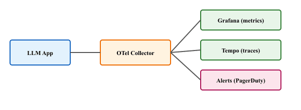
Grafana is the most common dashboard tool for OTel data. With Grafana Tempo for traces and Prometheus (or Mimir) for metrics, you can build unified dashboards that correlate latency spikes with token usage anomalies. The following example shows how to define custom OTel metrics that power these dashboards.
from opentelemetry import metrics
from opentelemetry.sdk.metrics import MeterProvider
from opentelemetry.sdk.metrics.export import PeriodicExportingMetricReader
from opentelemetry.exporter.otlp.proto.grpc.metric_exporter import OTLPMetricExporter

# Set up metrics export
metric_reader = PeriodicExportingMetricReader(
    OTLPMetricExporter(endpoint="http://otel-collector:4317"),
    export_interval_millis=10000, # Export every 10 seconds
    )
meter_provider = MeterProvider(metric_readers=[metric_reader])
metrics.set_meter_provider(meter_provider)

meter = metrics.get_meter("llm-app.operations")

# Define operational metrics
llm_latency = meter.create_histogram(
    "gen_ai.request.duration",
    unit="s",
    description="LLM request duration in seconds",
    )

llm_tokens = meter.create_counter(
    "gen_ai.tokens.consumed",
    description="Total tokens consumed by model and type",
    )

llm_errors = meter.create_counter(
    "gen_ai.errors",
    description="LLM API errors by type and model",
    )

active_requests = meter.create_up_down_counter(
    "gen_ai.requests.active",
    description="Currently in-flight LLM requests",
    )

# Usage in application code
import time

async def monitored_llm_call(model, messages, **kwargs):
    """LLM call with full metrics instrumentation."""
    labels = {"model": model, "provider": "openai"}
    active_requests.add(1, labels)
    start = time.monotonic()

    try:
        response = await client.chat.completions.create(
            model=model, messages=messages, **kwargs
            )
        duration = time.monotonic() - start
        llm_latency.record(duration, labels)
        llm_tokens.add(response.usage.prompt_tokens,
            {**labels, "token_type": "input"})
        llm_tokens.add(response.usage.completion_tokens,
            {**labels, "token_type": "output"})
        return response

    except Exception as e:
        llm_errors.add(1, {**labels, "error_type": type(e).__name__})
        raise

    finally:
active_requests.add(-1, labels)A well-designed LLM operations dashboard typically includes four panels: (1) a latency panel showing P50, P95, and P99 latency by model, with alerting thresholds; (2) a token consumption panel showing input and output tokens per hour, broken down by model and feature; (3) an error rate panel showing errors by type (rate limit, timeout, server error) with trend lines; and (4) a cost panel showing estimated spend per hour and projected monthly cost. The drift monitoring from Section 44.6 adds a fifth dimension: quality metrics derived from automated evaluation scores.
Objective
Set up a complete experiment tracking workflow using MLflow. You will first build a manual logging harness (the "right tool" baseline for understanding what gets tracked), then use MLflow's autologging and model registry features. By the end, you will have multiple tracked runs that you can compare in the MLflow UI.
What You'll Practice
- Setting up MLflow tracking with a local backend
- Logging parameters, metrics, and artifacts to experiment runs
- Comparing runs across hyperparameter configurations
- Registering and versioning model artifacts in the MLflow Model Registry
Setup
Install MLflow and a lightweight model library for the experiment.
Steps
Step 1: Manual experiment logging (from scratch)
Before relying on MLflow, build a simple JSON-based logging harness to understand what experiment tracking actually records. This makes the value of a dedicated tracking server concrete.
import json
import time
from datetime import datetime
from pathlib import Path

class ManualTracker:
    """A minimal experiment tracker using JSON files."""

    def __init__(self, experiment_dir="manual_experiments"):
        self.dir = Path(experiment_dir)
        self.dir.mkdir(exist_ok=True)

    def log_run(self, params, metrics, artifacts=None):
        run_id = f"run_{int(time.time())}"
        record = {
            "run_id": run_id,
            "timestamp": datetime.now().isoformat(),
            "params": params,
            "metrics": metrics,
            "artifacts": artifacts or [],
            }
        path = self.dir / f"{run_id}.json"
        path.write_text(json.dumps(record, indent=2))
        print(f"Logged run {run_id}: accuracy={metrics.get('accuracy', 'N/A')}")
        return run_id

    def compare_runs(self):
        runs = []
        for f in sorted(self.dir.glob("run_*.json")):
            runs.append(json.loads(f.read_text()))
            print(f"\n{'Run ID':<20} {'Accuracy':<10} {'Params'}")
            print("-" * 60)
            for r in runs:
                acc = r["metrics"].get("accuracy", "N/A")
                print(f"{r['run_id']:<20} {acc:<10.4f} {r['params']}")
                return runs

                # Quick test
                tracker = ManualTracker()
                tracker.log_run(
                    params={"model": "logistic_regression", "C": 1.0},
                    metrics={"accuracy": 0.85, "f1": 0.83},
                    )
                tracker.log_run(
                    params={"model": "logistic_regression", "C": 0.1},
                    metrics={"accuracy": 0.82, "f1": 0.80},
                    )
tracker.compare_runs()Step 2: Set up MLflow and log experiments
Now switch to MLflow for proper experiment tracking with a UI, artifact storage, and run comparison.
import mlflow
from sklearn.datasets import load_iris
from sklearn.model_selection import train_test_split
from sklearn.linear_model import LogisticRegression
from sklearn.metrics import accuracy_score, f1_score

# Configure MLflow (local file-based tracking)
mlflow.set_tracking_uri("file:./mlruns")
mlflow.set_experiment("iris-classification")

# Load data
X, y = load_iris(return_X_y=True)
X_train, X_test, y_train, y_test = train_test_split(
    X, y, test_size=0.2, random_state=42
    )

# Run experiments with different hyperparameters
for C_value in [0.01, 0.1, 1.0, 10.0]:
    with mlflow.start_run(run_name=f"logreg_C={C_value}"):
        # Log parameters
        mlflow.log_param("model_type", "LogisticRegression")
        mlflow.log_param("C", C_value)
        mlflow.log_param("solver", "lbfgs")

        # Train
        model = LogisticRegression(C=C_value, solver="lbfgs", max_iter=200)
        model.fit(X_train, y_train)

        # Evaluate
        preds = model.predict(X_test)
        acc = accuracy_score(y_test, preds)
        f1 = f1_score(y_test, preds, average="weighted")

        # Log metrics
        mlflow.log_metric("accuracy", acc)
        mlflow.log_metric("f1_weighted", f1)

        # Log the model as an artifact
        mlflow.sklearn.log_model(model, "model")

print(f"C={C_value:>5}: accuracy={acc:.4f}, f1={f1:.4f}")Step 3: Compare runs and identify the best model
Use the MLflow search API to query runs programmatically and find the best-performing configuration.
import mlflow
import pandas as pd
# Query all runs from the experiment
experiment = mlflow.get_experiment_by_name("iris-classification")
runs_df = mlflow.search_runs(
experiment_ids=[experiment.experiment_id],
order_by=["metrics.accuracy DESC"],
)
# Display comparison table
cols = ["run_id", "params.C", "metrics.accuracy", "metrics.f1_weighted"]
available = [c for c in cols if c in runs_df.columns]
print(runs_df[available].to_string(index=False))
# Identify best run
best_run = runs_df.iloc[0]
print(f"\nBest run: {best_run['run_id']}")
print(f" C = {best_run['params.C']}")
print(f" Accuracy = {best_run['metrics.accuracy']:.4f}")
print(f" F1 = {best_run['metrics.f1_weighted']:.4f}")Step 4: Register the best model
Promote the best model to the MLflow Model Registry, assigning it a version and stage label for deployment tracking.
import mlflow
# Register the best model
best_run_id = best_run["run_id"]
model_uri = f"runs:/{best_run_id}/model"
result = mlflow.register_model(model_uri, "iris-classifier")
print(f"Registered model: {result.name}, version: {result.version}")
# Transition to staging
from mlflow.tracking import MlflowClient
client = MlflowClient()
client.transition_model_version_stage(
name="iris-classifier",
version=result.version,
stage="Staging",
)
print(f"Model version {result.version} transitioned to Staging")
# Load and verify the registered model
loaded_model = mlflow.sklearn.load_model(
f"models:/iris-classifier/Staging"
)
verify_preds = loaded_model.predict(X_test)
verify_acc = accuracy_score(y_test, verify_preds)
print(f"Verified accuracy from registry: {verify_acc:.4f}")
print("\nTo view the UI, run: mlflow ui --port 5000")Stretch Goals
- Add MLflow autologging (
mlflow.sklearn.autolog()) and compare the captured metrics with your manual logging. - Log a confusion matrix plot as an artifact using
mlflow.log_figure()and view it in the MLflow UI. - Set up a model promotion workflow: automatically transition a model from Staging to Production only if its accuracy exceeds a threshold.
- OpenTelemetry provides the standardized observability backbone for LLM applications, with GenAI Semantic Conventions defining a common vocabulary for LLM telemetry.
- Auto-instrumentation libraries (OpenLLMetry, Traceloop) add tracing to LLM calls with minimal code changes, capturing token counts, model IDs, and latency automatically.
- Trace propagation through agent chains connects multi-step LLM workflows into a single trace, making it possible to debug complex agent behaviors end to end.
- Token tracking and cost attribution use OTel span attributes to allocate LLM costs to specific features, teams, or customers.
- Custom OTel dashboards for LLM operations should track p50/p95/p99 latency, tokens per second, cost per request, and error rates by model and endpoint.
Exercises
Set up OpenTelemetry tracing for a simple LLM application that makes a single chat completion call. Export traces to the console using ConsoleSpanExporter. Verify that the span includes the model name, token counts, and latency.
Answer Sketch
Initialize a TracerProvider with a SimpleSpanProcessor(ConsoleSpanExporter()). Create a span with tracer.start_as_current_span("gen_ai.chat"), set attributes for model and tokens after the API call, and verify the output includes all expected fields. The console output will show the span as a JSON object with the attributes you set.
Instrument a RAG pipeline with nested spans for embedding, vector search, and generation. Use a trace visualization tool (Jaeger or the console exporter) to verify that the spans form a proper parent-child hierarchy.
Answer Sketch
Create a parent span rag.pipeline, then use tracer.start_as_current_span() for each sub-step inside the parent's with block. OTel automatically links child spans to the active parent via context propagation. In Jaeger, you should see a waterfall view with the pipeline span at the top and sub-steps nested beneath it.
Build a multi-tenant cost attribution system using OTel metrics. Create counters for token usage and cost, labeled by tenant ID and feature name. Set up a Grafana dashboard (or equivalent) that shows per-tenant cost breakdown and alerts when any tenant exceeds their monthly budget.
Answer Sketch
Use the TokenTracker pattern from Code Fragment 42.9.4a. Add tenant and feature labels to all metric emissions. In Grafana, create a panel with PromQL: sum by (tenant_id)(rate(gen_ai_cost_usd_total[1h])) * 720 to project monthly costs. Set alert rules on the projected cost exceeding per-tenant thresholds.
Design a content redaction strategy for OTel traces in a healthcare chatbot application subject to HIPAA. Specify which span attributes should be captured, which should be redacted, and how to handle trace storage and retention.
Answer Sketch
Capture: model name, token counts, latency, error types, feature name. Redact: all prompt content, completion content, and user identifiers. Use an OTel Collector processor to strip sensitive attributes before export. Store traces in a HIPAA-compliant backend with encryption at rest and access logging. Set retention to the minimum required for operational debugging (7 to 30 days). Never include PHI in span attributes or events.
What Comes Next
In the next chapter, Chapter 62: LLMOps & Deployment Engineering, we move from observability to the deployment, scaling, and operational patterns that bring LLM applications to production. The OTel instrumentation you learned here becomes the foundation for monitoring those production systems.
For the online-evaluation and drift-detection workflows that consume OpenTelemetry traces, see Section 66.2: Online Evaluation and Observability. For the LangSmith, Langfuse, and Arize Phoenix platforms that wrap OTel for LLM apps, see Section 45.2: Observability Tools. For the agent-trace evaluation patterns (multi-step reasoning, tool-call grading) built on the same span model, see Section 43.1: RAG Evaluation.